Python-linear regression
This is the 184th article of the running keyboard man
Author|I am a running keyboard man
Source | Running Keyboard Hero (ID: runningkeyboardhero)
Please contact authorization for reprinting (WeChat ID: ctwott)
After tossing for a long time, I think I still need to record something, whether it is for reference to interested friends or to deepen my own learning and understanding, it will be beneficial.
However, I have been thinking about this topic for a long time. I have deep learning in the professional direction. I am currently gnawing on machine learning.
Simply put this series into Python.
Of course, the content of this section must be high-energy! ! !
Anyway, this month’s time is spent, one week to learn a, one week to learn b, and then take some time to smooth the whole process...
The basic content is directly linked:
Python-matplotlib drawing (not annoying notes)
Chenkc, public number: AI machine learning and deep learning algorithms [simple drawing with matplotlib] (http://mp.weixin.qq.com/s?__biz=Mzg5NzE1NzM4NA==&mid=2247484802&idx=1&sn=c57b5913d82b743b8d386484de25058e&chksm=c07755e5f700dcf38230415c902df49c33ec48e1feac222902f59083177537b99f5f23edb40b#rd)
Know the link https://www.zhihu.com/collection/260736383
Explain the profound things in a simple way--gradient descent method and its implementation, the short book link: https://www.jianshu.com/p/c7e642877b0e
With the previous two foreshadowing, you can directly upload the code
#! /usr/bin/env python3.6
# - *- coding: utf-8-*-
# @ Time    :2020-11-0712:22
# @ Author  : Ed Frey
# @ File    : linear_regression.py
# @ Software: PyCharm

import matplotlib.pyplot as plt
import numpy as np

m =20
X0 = np.ones((m,1))
X1 = np.arange(1, m +1).reshape(m,1)
X = np.hstack((X0, X1))
y = np.array([3,4,5,5,2,4,7,8,11,8,12,11,13,13,16,17,18,17,19,21]).reshape(m,1)
xx = X1.reshape(1, m)[0]
yy = y.reshape(1, m)[0]
fig = plt.figure(figsize=(12,10), dpi=80)
plt.ion()

alpha =0.01
def error_function(theta, X, y):
 diff = np.dot(X, theta)- y
 return(1./2* m)* np.dot(np.transpose(diff), diff)

def gradient_function(theta, X, y):
 diff = np.dot(X, theta)- y
 return(1./ m)* np.dot(np.transpose(X), diff)

def gradient_descent(X, y, alpha):
 theta = np.array([1,1]).reshape(2,1)
 gradient =gradient_function(theta, X, y)

 i =0
 items =[]while not np.all(np.absolute(gradient)<=1e-5):
  theta = theta - alpha * gradient
  gradient =gradient_function(theta, X, y)
  u = np.linspace(-1,22,20)
  v = theta[0][0]+ theta[1][0]* u
  i +=1if i %1000==1:
   items.append(theta)
 items.append(theta)
 j =0for theta in items:
  plt.cla()
  j +=1
  plt.title("linear %s"%j)
  plt.scatter(xx, yy)
  plt.grid(True)
  ax = plt.gca()
  ax.spines['right'].set_color('none')
  ax.spines['top'].set_color('none')
  ax.xaxis.set_ticks_position('bottom')
  ax.spines['bottom'].set_position(('data',0))
  ax.yaxis.set_ticks_position('left')
  ax.spines['left'].set_position(('data',0))
  plt.xlim(-2,30,20)
  plt.ylim(-2,30,20)
  u0 =20
  v0 = theta[0][0]+ theta[1][0]* u0
  plt.plot(u, v, linewidth=3.0, color='r')
  plt.annotate(r'$%f*u + %f = v$'%(theta[1][0], theta[0][0]), xy=(u0, v0), xycoords='data',
      xytext=(-200,20), textcoords='offset points', fontsize=16,
      arrowprops=dict(arrowstyle='->', connectionstyle='arc3,rad=.2'))
  plt.savefig(fname="scatter%s.png"%j)
  plt.pause(1)return theta

plt.ioff()
plt.show()
optimal =gradient_descent(X, y, alpha)print('optimal:', optimal)print('error function:',error_function(optimal, X, y)[0,0])
The code is not explained too much, it is basically copied from the short book, and the explanation above is sufficiently detailed. What's unfamiliar to novices is the representation of matrices and coordinates. For example, two N*1 dimensional matrices, a and b, are converted into coordinates. The abscissas are all in a and the ordinates are in b. As for the gradient descent method, it is the basic part of mathematical analysis. In addition, it involves a little bit of knowledge of matrix operations, and I got a little card at the time.
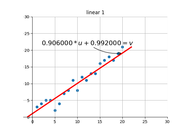
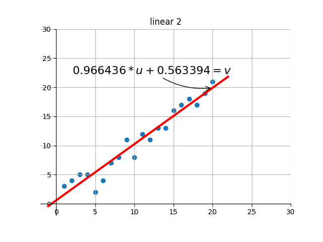
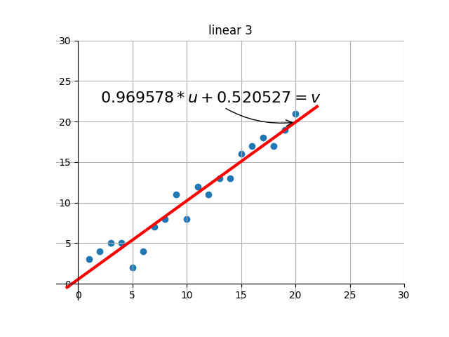
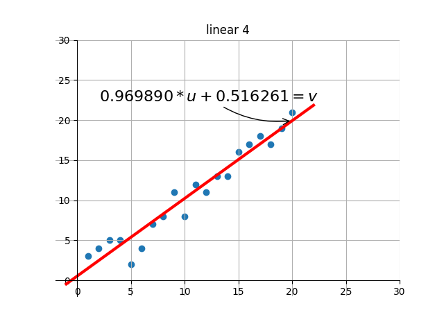
The code in the drawing part is supplemented and designed by myself. The basic function is to visualize the effect of the current solution in the process of iteratively searching for the optimal solution of the target, that is, to view the linear effect corresponding to the current parameter through the graph.
Intercepted several renderings of the output:
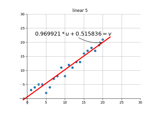
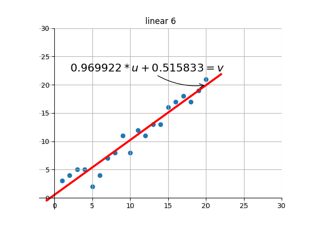
what? Didn't you feel it? Let's have another animation

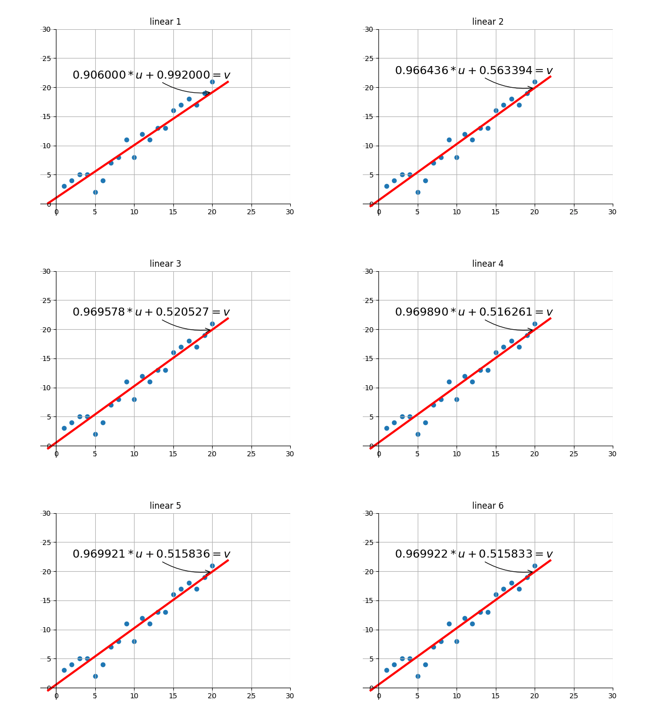
- END-
Recommended Posts