Python binomial distribution, Poisson distribution

Click to follow not to get lost

lead

Speak

Knock on the blackboard, dry goods have reached the battlefield! ! ! In data analysis, binomial distribution and Poisson distribution are the two distributions we often use. Today, I will briefly introduce the basis of binomial distribution: Bernoulli test, n-fold Bernoulli test and two-point distribution Next, let’s explain the concepts of binomial distribution and Poisson distribution. After that, let’s explain the conditions for the conversion of the binomial distribution to the Poisson distribution. Finally, let’s see through python why the binomial distribution can be converted to Poisson under certain conditions. The loose distribution is approximated.

Bernoulli test

I believe that everyone has tossed a coin. When there is a coin toss, there are only two results, whether it is a positive or a negative, in fact, a test like this is a Bernoulli test. Now let’s make an abstract summary: suppose a random test E has only two results, event A appears and event A does not appear. At the same time, the probability of event A appearing is p, and the probability of not appearing is q, 0 <p<1,q=1-p,这样的一次试验我们把它叫做伯努利试验。将伯努利试验进行n重独立实验，重复做n次，这样的n重独立实验就是n重伯努利试验。

Two-point distribution

The distribution corresponding to the Bernoulli test is a two-point distribution, which is also called a 0-1 distribution, that is, the distribution of a random variable X is listed as:

Note: 1 represents the probability of occurrence, 0 represents the probability of not occurring

Binomial distribution

In the n-fold Bernoulli experiment, the corresponding distribution of the number of occurrences of event A is binomial distribution, that is, the distribution of random variable X is listed as:

Where 0 <p<1,q=1-p,当n=1时，二项分布就是两点分布。

Poisson distribution

The Poisson distribution comes from the name of the mathematician Simeon Denis-Poisson (1781-1840). The Poisson distribution is mainly used to measure the number of discrete events in continuous time or space. The formula is as follows:

λ>0 means the average number of occurrences. If the random variable obeys the binomial distribution, and

In other words, when n is large and p is small, the Poisson distribution can be used to approximate the binomial distribution to solve the problem. Why?

First of all, the things mentioned above actually have a formal name called Poisson's Theorem. Since it is a theorem, it means that the above things must be established. Next, let’s look at an easy-to-understand example. Here is why.

Let's take the question of how many babies will be born in the hospital in one day (this question obeys the Poisson distribution) as an example:

We can take this day's time with the limit of thinking, and subdivide it into n small time periods infinitely. In each small time period, are there only two results: the baby is born and the baby is not born, is this one? We can regard a small period of time as a random experiment, and the results of the test are only two births and no births, so whether n small time periods can be regarded as an n-fold Bernoulli test, using distribution To describe: It is a binomial distribution. Is the Poisson distribution transformed into a binomial distribution? So in simple terms, when n is large and p is small, the binomial distribution is the Poisson distribution, and the Poisson distribution is the binomial distribution. Of course, it can be approximated instead.

Next, we use a computer to simulate this result.

**Note: Generally, when n>=20 and p<=0.05, the Poisson distribution can be used to approximate the binomial distribution. **

01

python implementation

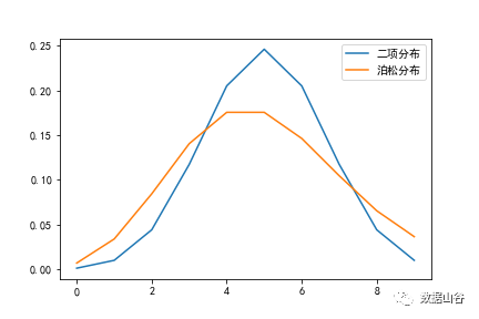
When n is 10 and p=0.5, according to the above conditions, we know that the binomial distribution should not be approximated by the Poisson distribution. The figure below shows that when n is 10 and p=0.5, the binomial distribution and Poisson distribution are also Obviously different (see below for specific code)

# Import the corresponding library
import numpy as np
import pandas as pd
import matplotlib.pyplot as plt
from scipy import stats
# Plot binomial distribution and Poisson distribution
n =10
p=0.5
q=1-p
bino = stats.binom(n,p)
x = np.arange(0,n)
y1 = bino.pmf(x)
possion = stats.poisson(n*p)
y2 = possion.pmf(x)
plt.plot(x,y1,label="Binomial distribution")
plt.plot(x,y2,label="Poisson distribution")
plt.legend()
plt.show()

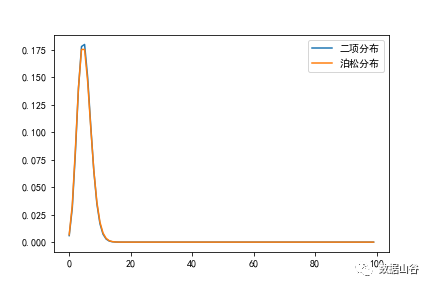
When n is 100 and p=0.05, according to the above conditions, we know that the binomial distribution should be approximately replaced by Poisson distribution. The figure below shows that when n is 100 and p=0.05, the binomial distribution and Poisson distribution are Very similar (see below for specific code)

# Import the corresponding library
import numpy as np
import pandas as pd
import matplotlib.pyplot as plt
from scipy import stats
# Draw binomial distribution diagram and Poisson distribution diagram
n =100
p=0.05
q=1-p
bino = stats.binom(n,p)
x = np.arange(0,n)
y1 = bino.pmf(x)
possion = stats.poisson(n*p)
y2 = possion.pmf(x)
plt.plot(x,y1,label="Binomial distribution")
plt.plot(x,y2,label="Poisson distribution")
plt.legend()
plt.show()

02

to sum up

Today we mainly learned what is called the binomial distribution, the Poisson distribution, and the approximate replacement of the Poisson distribution for the binomial distribution. I believe everyone should have already understood the relationship between the two. In the next section, we focus on the binomial distribution and the normal distribution, and reveal what kind of "love and hatred" there will be between them, so stay tuned!