Hyperparameter optimization using Python
The code attached to this article can be found here.
https://github.com/NMZivkovic/ml_optimizers_pt3_hyperparameter_optimization
So far, in the whole process of learning machine learning, several major topics have been covered. Researched some regression algorithms, classification algorithms and algorithms that can be used for two types of problems (SVM, decision tree and random forest). In addition, I immersed toes in unsupervised learning, learned how to use this type of learning for clustering, and learned about several clustering techniques. In all these articles, Python is used to implement "from scratch" and libraries such as TensorFlow, Pytorch and SciKit Learn.

Worried that AI will take over your work? Make sure it is the one who built it. Stay relevant to the rising AI industry!
Hyperparameters are an integral part of every machine learning and deep learning algorithm. Unlike the standard machine learning parameters learned by the algorithm itself (such as w and b in linear regression or connection weights in neural networks), engineers set hyperparameters before the training process. They are external factors that control the behavior of the learning algorithm fully defined by the engineer. Need some examples?
The learning rate is one of the most famous hyperparameters. C is also a hyperparameter in SVM. The maximum depth of the decision tree is a hyperparameter, etc. These can be manually set by engineers. But if you want to run multiple tests, it may be troublesome. That's where hyperparameter optimization is used. The main goal of these techniques is to find the hyperparameters of a given machine learning algorithm that can provide the best performance measured on the validation set. In this tutorial, several techniques that can provide the best hyperparameters are explored.
Data set and prerequisites
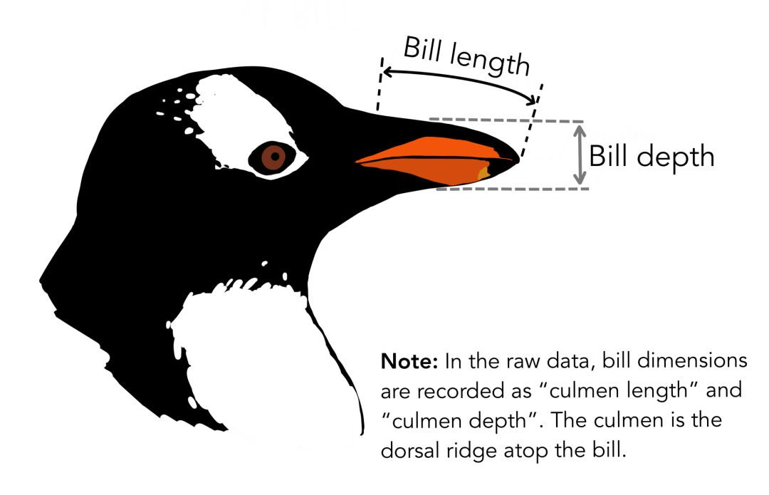
The data used in this article comes from the PalmerPenguins dataset. This data set was recently introduced to replace the famous Iris data set. It was created by Dr. Kristen Gorman and Palmer Station in Antarctica. You can get this dataset here or through Kaggle. This data set essentially consists of two data sets, each of which contains data for 344 penguins. Just like in the iris data set, there are 3 different penguins in the 3 islands of the Palmer Islands. Again, these data sets contain specimen dimensions for each species. The high gate is the upper ridge of the beak. In the simplified penguin data, the vertex length and depth have been renamed to the culmen_length_mm and culmen_depth_mm variables.
https://github.com/allisonhorst/palmerpenguins
Since the data set has been labeled, it will be able to verify the experimental results. But this is usually not the case, and the verification of clustering algorithm results is usually a difficult and complex process.
For the purposes of this article, please ensure that the following Python libraries are installed:
- NumPy
- SciKit learning
- SciPy
- Sci-Kit optimization
After the installation is complete, make sure you have imported all the necessary modules used in this tutorial.
import pandas as pd
import numpy as np
import matplotlib.pyplot as plt

from sklearn.preprocessing import StandardScaler
from sklearn.model_selection import train_test_split
from sklearn.metrics import accuracy_score

from sklearn.model_selection import GridSearchCV, RandomizedSearchCV

from sklearn.svm import SVC
from sklearn.ensemble import RandomForestRegressor

from scipy import stats
from skopt import BayesSearchCV
from skopt.space import Real, Categorical
In addition, at least familiar with the basics of linear algebra, calculus and probability.
Prepare data
Load and prepare the PalmerPenguins data set. First load the data set and delete the unused functions in this article:
data = pd.read_csv('./data/penguins_size.csv')

data = data.dropna()
data = data.drop(['sex','island','flipper_length_mm','body_mass_g'], axis=1)
Then separate the input data and scale it:
X = data.drop(['species'], axis=1)

ss =StandardScaler()
X = ss.fit_transform(X)

y = data['species']
spicies ={'Adelie':0,'Chinstrap':1,'Gentoo':2}
y =[spicies[item]for item in y]
y = np.array(y)
Finally, the data is divided into training and test data sets:
X_train, X_test, y_train, y_test =train_test_split(X, y, test_size=0.2, random_state=33)
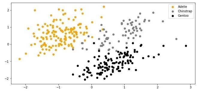
When plotting the data, here is what it looks like:
Grid search
Manual hyperparameter adjustment is slow and annoying. This is why we explored the first and simplest hyperparameter optimization technique-grid search. This technology is accelerating the process, and it is one of the most commonly used hyperparameter optimization techniques. Essentially, it automates the trial and error process. For this technique, a list of all hyperparameter values is provided, and the algorithm builds a model for each possible combination, evaluates it, and then selects the value that provides the best result. This is a general technique that can be applied to any model.

In the example, the SVM algorithm is used for classification. Three hyperparameters C, gamma and kernel are considered. To learn more about them, check out this article. For C, check the following values: 0.1, 1, 100, 1000; for gamma, use values: 0.0001, 0.001, 0.005, 0.1, 1, 3, 5; for kernel, use values:'linear' and'rbf'. This is what it looks like in the code:
hyperparameters ={'C':[0.1,1,100,1000],'gamma':[0.0001,0.001,0.005,0.1,1,3,5],'kernel':('linear','rbf')}
Use Sci-Kit Learn and its SVC class, which contains the SVM implementation for classification. In addition, use the GridSearchCV class, which is used for grid search optimization. The combination looks like this:
grid =GridSearchCV(
  estimator=SVC(),
  param_grid=hyperparameters,
  cv=5,
scoring='f1_micro',
n_jobs=-1)
This class receives several parameters through the constructor:
- Estimator-instance machine learning algorithm itself. A new instance of the SVC class is passed there.
- param_grid-contains a dictionary of hyperparameters.
- cv-Determine the cross-validation split strategy.
- Scoring-a verification indicator used to evaluate predictions. Use F1 scores.
- n_jobs-indicates the number of jobs to run in parallel. The value -1 means that all processors are in use.

The only thing left to do is to run the training process by using the fit method:
grid.fit(X_train, y_train)
After training, you can check the best hyperparameters and the scores of these parameters:
print(f'Best parameters: {grid.best_params_}')print(f'Best score: {grid.best_score_}')
Best parameters:{'C':1000,'gamma':0.1,'kernel':'rbf'}
Best score:0.9626834381551361
Similarly, you can print out all the results:
print(f'All results: {grid.cv_results_}')
-
Allresults: {'mean_fit_time': array([0.00780015, 0.00280147, 0.00120015, 0.00219998, 0.0240006 ,*
-
0.00739942, 0.00059962, 0.00600033, 0.0009994 , 0.00279789,* -
0.00099969, 0.00340114, 0.00059986, 0.00299864, 0.000597 ,* -
0.00340023, 0.00119658, 0.00280094, 0.00060058, 0.00179944,* -
0.00099964, 0.00079966, 0.00099916, 0.00100031, 0.00079999,* -
0.002 , 0.00080023, 0.00220037, 0.00119958, 0.00160012,* -
0.02939963, 0.00099955, 0.00119963, 0.00139995, 0.00100069,* -
0.00100017, 0.00140052, 0.00119977, 0.00099974, 0.00180006,* -
0.00100312, 0.00199976, 0.00220003, 0.00320096, 0.00240035,* -
0.001999 , 0.00319982, 0.00199995, 0.00299931, 0.00199928, *
...
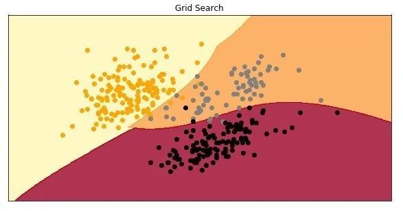
Okay, now build this model and check how it performs on the test data set:
model =SVC(C=500, gamma =0.1, kernel ='rbf')
model.fit(X_train, y_train)

preditions = model.predict(X_test)print(f1_score(preditions, y_test, average='micro'))
0.9701492537313433
Cool, the accuracy of the model using the suggested hyperparameters is about 97%. This is how it looks when the model is drawn:
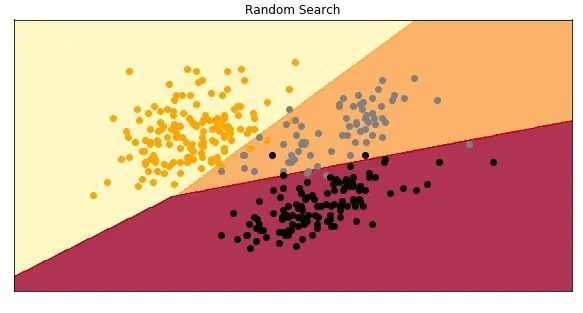
Random search
Grid search is very simple. But it is also computationally expensive. Especially in the field of deep learning, training may take a lot of time. Likewise, some hyperparameters may be more important than others. This is why the idea of random search was born in the introduction of this article. In fact, this study shows that in terms of computational cost, random search is more effective than grid search for hyperparameter optimization. This technique also allows more precise discovery of good values for important hyperparameters.

Just like Grid Search, Random Search creates a grid of hyperparameter values and selects random combinations to train the model. This method may miss the best combination, but compared to Grid Search, it unexpectedly selects the best result more frequently and takes very little time. See how it works in the code. Same=Use Sci-Kit Learn's SVC class, but this time use RandomSearchCV class for random search optimization.
hyperparameters ={"C": stats.uniform(500,1500),"gamma": stats.uniform(0,1),'kernel':('linear','rbf')}

random =RandomizedSearchCV(
    estimator =SVC(),
    param_distributions = hyperparameters,
    n_iter =100,
    cv =3,
    random_state=42,
    n_jobs =-1)

random.fit(X_train, y_train)
Note that a uniform distribution is used for C and gamma. The result can also be printed out:
print(f'Best parameters: {random.best_params_}')print(f'Best score: {random.best_score_}')
-
Best parameters: {'C': 510.5994578295761, 'gamma': 0.023062425041415757, 'kernel': 'linear'}*
-
Best score: 0.9700374531835205*
Please note that it is close but the result is different from when using Grid Search. The value of the hyperparameter C of the grid search is 500, and the value of the hyperparameter C of the random search is 510.59. With this item alone, you can see the benefits of random search, because it is unlikely to put this value in the grid search list. Similarly, for gamma, random search yields 0.23, while grid search yields 0.1. What is really surprising is that Random Search chose a linear kernel instead of RBF and achieved a higher F1 score. To print all results, use the cv_results_ attribute:
print(f'All results: {random.cv_results_}')
-
Allresults: {'mean_fit_time': array([0.00200065, 0.00233404, 0.00100454, 0.00233777, 0.00100009,*
-
0.00033339, 0.00099715, 0.00132942, 0.00099921, 0.00066725,* -
0.00266568, 0.00233348, 0.00233301, 0.0006667 , 0.00233285,* -
0.00100001, 0.00099993, 0.00033331, 0.00166742, 0.00233364,* -
0.00199914, 0.00433286, 0.00399915, 0.00200049, 0.01033338,* -
0.00100342, 0.0029997 , 0.00166655, 0.00166726, 0.00133403,* -
0.00233293, 0.00133729, 0.00100009, 0.00066662, 0.00066646,* -
....*
Do the same thing as Grid Search: create a model with the suggested hyperparameters, check the scores of the test data set and draw the model.
model =SVC(C=510.5994578295761, gamma =0.023062425041415757, kernel ='linear')
model.fit(X_train, y_train)

preditions = model.predict(X_test)print(f1_score(preditions, y_test, average='micro'))
0.9701492537313433
The F1 score on the test data set is exactly the same as the score when using grid search. View the model:
Bayesian optimization
A very cool fact about the first two algorithms is that all experiments with different hyperparameter values can be run in parallel. This can save a lot of time. However, this is also their biggest shortcoming. This means that since each experiment is conducted independently, information from past experiments cannot be used in the current experiment. The entire field is dedicated to solving the problem of sequence optimization-Sequence Model-Based Optimization (SMBO). The algorithms explored in this field use previous experiments and observations of the loss function. Based on them, try to determine the next best point. Bayesian optimization is one of such algorithms.

Just like other algorithms from the SMBO group, the previously evaluated points (in this case, they are hyperparameter values, but we can generalize) are used to calculate the posterior expectation of the loss function. The algorithm uses two important mathematical concepts-Gaussian process and acquisition function. Since the Gaussian distribution is done on random variables, the Gaussian process is a generalization of the function. Just as the Gaussian distribution has a mean and a covariance, the Gaussian process is described by a mean function and a covariance function.
The acquisition function is a function used to evaluate the current loss value. One way to observe it is to use it as a loss function. It is a function of the posterior distribution of the loss function and describes the utility of all values of hyperparameters. The most popular collection functions are expected to improve:
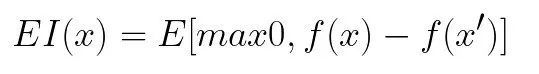
Where f is the loss function and x'is the current best hyperparameter set. When putting all these together, Byesian optimization is done in 3 steps:
- Using the previously evaluated loss function points, a Gaussian process is used to calculate the posterior expectation.
- A new point set that maximizes the expected improvement effect is selected
- Calculate the loss function of the newly selected point

The easy way to introduce it into the code is to use the Sci-Kit optimization library, usually called skopt. Following the procedure used in the previous example, you can do the following:
hyperparameters ={"C":Real(1e-6,1e+6, prior='log-uniform'),"gamma":Real(1e-6,1e+1, prior='log-uniform'),"kernel":Categorical(['linear','rbf']),}

bayesian =BayesSearchCV(
    estimator =SVC(),
    search_spaces = hyperparameters,
    n_iter =100,
    cv =5,
    random_state=42,
    n_jobs =-1)

bayesian.fit(X_train, y_train)
Similarly, a dictionary is defined for the hyperparameter set. Please note that the Real and Categorical classes in the Sci-Kit Optimization library are used. Then use the BayesSearchCV class in the same way as using GridSearchCV or RandomSearchCV. After training, you can print out the best results:
print(f'Best parameters: {bayesian.best_params_}')print(f'Best score: {bayesian.best_score_}')
-
Best parameters:*
-
OrderedDict([('C', 3932.2516133086), ('gamma', 0.0011646737978730447), ('kernel', 'rbf')])*
-
Best score: 0.9625468164794008*
Using this optimization, we got very different results. The loss is higher than when using random search. You can even print all results:
print(f'All results: {bayesian.cv_results_}')
-
All results: defaultdict(<class 'list'>, {'split0_test_score': [0.9629629629629629,*
-
0.9444444444444444, 0.9444444444444444, 0.9444444444444444, 0.9444444444444444,*
-
0.9444444444444444, 0.9444444444444444, 0.9444444444444444, 0.46296296296296297,*
-
0.9444444444444444, 0.8703703703703703, 0.9444444444444444, 0.9444444444444444,*
-
0.9444444444444444, 0.9444444444444444, 0.9444444444444444, 0.9444444444444444,*
-
.....*
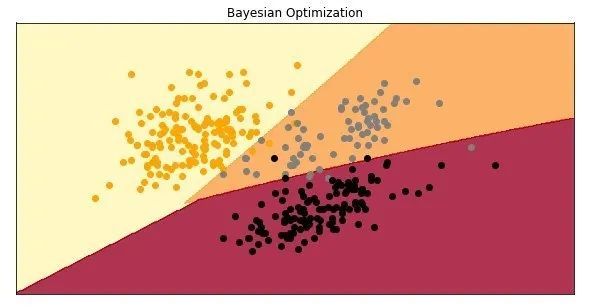
How does the model with these hyperparameters perform on the test data set?
model =SVC(C=3932.2516133086, gamma =0.0011646737978730447, kernel ='rbf')
model.fit(X_train, y_train)

preditions = model.predict(X_test)print(f1_score(preditions, y_test, average='micro'))
0.9850746268656716
This is very interesting. Even if the results obtained on the validation data set are poor, they get better scores on the test data set. This is the model:
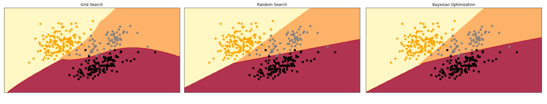
Just for fun, put all these models together:
Options
Usually the previously described method is the most popular and commonly used. But if the previous solution is not suitable, several alternative methods can be considered. One of them is the gradient-based optimization of hyperparameter values. This technique calculates the gradient of the relevant hyperparameters, and then uses the gradient descent algorithm to optimize it. The problem with this approach is that for gradient descent to work properly, it requires a convex and smooth function, which is usually not the case when talking about hyperparameters. Another method is to use evolutionary algorithms for optimization.
in conclusion
In this article, several well-known hyperparameter optimization and adjustment algorithms are introduced. Learned how to use grid search, random search and Bayesian optimization to obtain the best values of hyperparameters. I also saw how to use Sci-Kit Learn classes and methods in the code.
Recommended Posts