Least squares method and its python implementation details

Least Square Method, as the basis of classification regression algorithm, has a long history (proposed by Marie Legendre in 1806). It finds the best function match of the data by minimizing the sum of squares of errors. The least square method can be used to easily obtain unknown data, and minimize the sum of squares of errors between the obtained data and the actual data. The least square method can also be used for curve fitting. Some other optimization problems can also be expressed by the least square method by minimizing energy or maximizing entropy.

So what is the least square method? Don't worry, let's start with a few simple concepts.

Suppose we now have a series of data points

, Then the estimator obtained by the fitting function h(x) given by us is

, Then how to evaluate the high degree of fit between the fitting function we gave and the actual function to be solved? Here we first define a concept: residual

, We estimate that the degree of fit is based on the residuals. Here are three more norms:

• ∞-norm: the maximum value of the absolute value of the residual

, Which is the maximum value of residual distance among all data points

• 1-norm: sum of absolute residuals

, Which is the sum of residual distances of all data points

• 2-norm: sum of squared residuals

The first two norms are the easiest to think of and the most natural, but they are not conducive to differential calculations. When the amount of data is large, the amount of calculation is too large and it is not operability. Therefore, 2-norm is generally used.

Having said that, what is the relationship between norm and fitting? The degree of fitting, in popular terms, is the similarity between our fitting function h(x) and the function y to be solved. Then the smaller the 2-norm, the higher the natural similarity.

From this, we can write the definition of the least squares method:

For the given data

, In the given hypothesis space H, solve h(x)∈H so that the residual

Has the smallest 2-norm, that is

Geometrically speaking, it is to find and a given point

The curve with the smallest sum of squared distances is y=h(x). h(x) is called the fitting function or least square solution, and the method of solving the fitting function h(x) is called the least square method of curve fitting.

So what should h(x) look like here? In general, this is a polynomial curve:

Here h(x,w) is a polynomial of degree n, and w is its parameter.

In other words, the least square method is to find such a group

, Making

The smallest.

So how to find such w so that its fitting function h(x) has the highest degree of fitting with the objective function y? That is, how to solve the least squares method, this is the key.

Suppose our fitting function is a linear function, namely:

(Of course, it can also be a quadratic function, or a higher-dimensional function. This is just a solution example, so the simplest linear function is used) Then our goal is to find such w,

Here order

As a sample

Square loss function

Here Q(w) is the risk function we want to optimize.

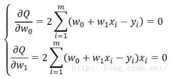
Students who have studied calculus should be clearer. This is a typical problem of solving extreme values. You only need to find the partial derivatives of 18 separately, and then set the partial derivatives to 0 to find the extreme points, namely:

Next, you only need to solve this system of equations to solve the value of w_i

============ Split split =============

Above we explained what the least squares method is and how to solve the least squares solution. Below we will implement the least squares method through Python.

Here we choose the objective function as y=sin(2πx), superimpose a normal distribution as noise interference, and then use a polynomial distribution to fit it.

Code:

# _*_ coding: utf-8 _*_
# Author: yhao
# Blog: http://blog.csdn.net/yhao2014
# mailbox: [email protected]
 
import numpy as np #Introduce numpy
import scipy as sp
import pylab as pl
from scipy.optimize import leastsq #Introduce the least square function
 
n =9 #Polynomial degree
 
 
# Objective function
def real_func(x):return np.sin(2* np.pi * x)
 
 
# Polynomial function
def fit_func(p, x):
 f = np.poly1d(p)returnf(x)
 
 
# Residual function
def residuals_func(p, y, x):
 ret =fit_func(p, x)- y
 return ret
 
 
x = np.linspace(0,1,9) #Randomly select 9 points as x
x_points = np.linspace(0,1,1000) #Consecutive points needed for drawing
 
y0 =real_func(x) #Objective function
y1 =[np.random.normal(0,0.1)+ y for y in y0] #Function after adding normal distribution noise
 
p_init = np.random.randn(n) #Randomly initialize polynomial parameters
 
plsq =leastsq(residuals_func, p_init, args=(y1, x))
 
print 'Fitting Parameters: ', plsq[0] #Output fitting parameters
 
pl.plot(x_points,real_func(x_points), label='real')
pl.plot(x_points,fit_func(plsq[0], x_points), label='fitted curve')
pl.plot(x, y1,'bo', label='with noise')
pl.legend()
pl.show()

Output fitting parameters:

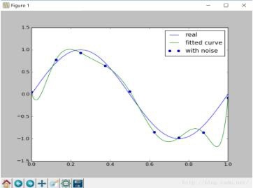
The image is as follows:

From the image, it is obvious that our fitting function is over-fitting. Next, we try to add a regularization term to the risk function to reduce the phenomenon of over-fitting:

For this, we only need to add lambda^(1/2)p to the returned array in the residual function

regularization =0.1 #Regularization coefficient lambda
 
 
# Residual function
def residuals_func(p, y, x):
 ret =fit_func(p, x)- y
 ret = np.append(ret, np.sqrt(regularization)* p) #Lambda^(1/2)p is added to the returned array
 return ret

Output fitting parameters:

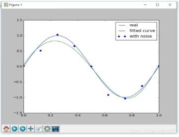
The image is as follows:

Obviously, under proper regularization constraints, the objective function can be better fitted.

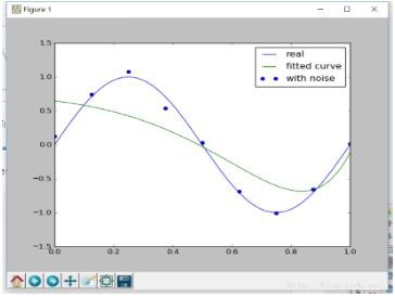
Note that if the coefficient of the regularization term is too large, it will lead to underfitting (the penalty term at this time has a particularly high weight)

For example, when setting regularization=0.1, the image is as follows:

At this time, it is obviously under-fitting. Therefore, the selection of regularization parameters must be carefully performed.

The above detailed explanation of the least squares method and its python implementation is all the content shared by the editor, I hope to give you a reference.