FM algorithm analysis and Python implementation

**1. What is FM? **

FM stands for Factor Machine, factorization machine.

**2. Why do we need FM? **

1、 Feature combination is a problem encountered in many machine learning modeling processes. If you model features directly, it is likely to ignore the associated information between features and features. Therefore, you can build a new cross feature feature combination Ways to improve the effect of the model.

2、 High-dimensional sparse matrix is a common problem in practical engineering, and directly leads to excessive calculation and slow update of feature weights. Imagine a 10000100 table with 8 elements in each column. After one-hot encoding, a 10000800 table will be generated. Therefore, in each row of the table, there are only 100 values of 1, and 700 values of 0.

The advantage of FM lies in the handling of these two issues. The first is feature combination. By combining pairwise features, cross-term features are introduced to improve the model score; the second is high-dimensional disaster, and the parameter estimation of features is completed by introducing hidden vectors (matrix decomposition of the parameter matrix).

**3. Where is FM used? **

We already know that FM can solve the problem of feature combination and high-dimensional sparse matrix. In actual business scenarios, the scenarios of e-commerce, Douban and other recommendation systems are the most widely used areas. For example, Xiao Wang has only browsed on Douban. 20 movies, and Douban has 20,000 movies. If you build a movie matrix based on Xiao Wang, there will be no doubt that there will be 199980 elements in it, all 0. And similar problems can be solved by FM.

**4. What does FM look like? **

Before showing the FM algorithm, let's review the most common linear expressions:

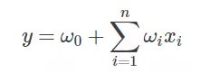
Where w0 is the initial weight, or understood as a bias term, and wi is the weight corresponding to each feature xi. It can be seen that this linear expression only describes the relationship between each feature and the output.

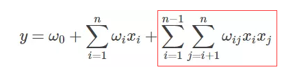
The expression of FM is as follows. It can be observed that only the new cross-term characteristics and corresponding weights are added after the linear expression.

5. Expansion of FM Intersections

5.1 Looking for cross terms###

The core of the solution of the FM expression lies in the solution of the cross term. The following is the expansion that many people use to solve the cross term. Those who are new to the FM algorithm may have doubts. I don't know how to expand the formula. Then I will derive it manually.

There are 3 variables (features) x1 x2 x3, and the hidden variables of each feature are v1=(1 2 3), v2=(4 5 6), v3=(1 2 1), namely:

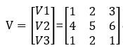
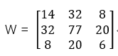
Let the weight matrix W composed of the cross terms be a symmetric matrix. The reason why it is set as a symmetric matrix is because the symmetric matrix can be replaced by a vector multiplied by a vector transpose.
Then W=VVT, namely

and so:

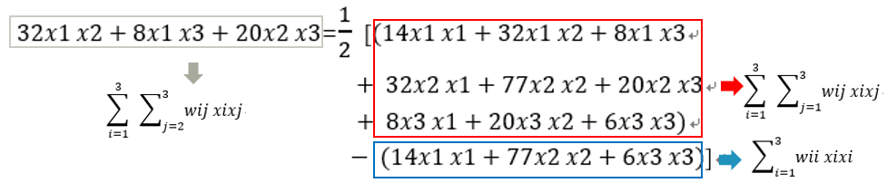
In fact, the cross term we should consider should be the term that excludes its own combination, that is, x1x1, x2x2, and x3x3 are not considered cross terms, then the real cross terms are x1x2, x1x3, x2x1, x2x3, x3x1, x3x2.
After deduplication, the cross terms are x1x2, x1x3, and x2x3. This is why 1/2 appears in the formula.

5.2 Cross item weight conversion###

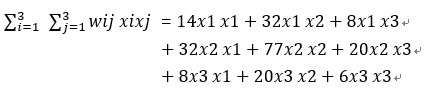
After you have a basic understanding of the cross terms, the formula will be decomposed below, taking n=3 as an example.

and so:

wij can be written as

or

, It depends on whether vi is a 13 or 31 vector.

5.3 Cross-term expansion###

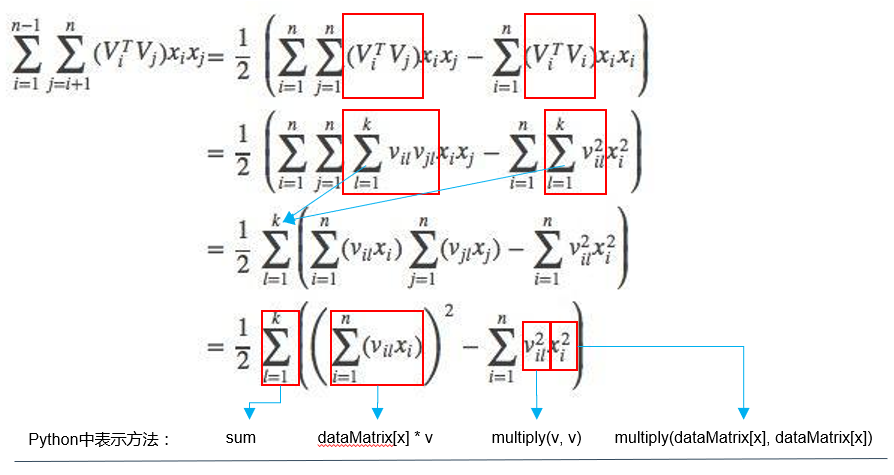
The above example is a cross-term derivation of 3 features, so for n features, the cross-term formula of FM can be generalized to:

We can further decompose:

So the cross term of the FM algorithm can finally be expanded into:

5.4 The hidden vector v is the embedding vector?

Suppose the shape of the training data set dataMatrix is (20000, 9), and one row of data is taken as a sample i, then the shape of the sample i is (1, 9), and the shape of the hidden vector vi is (9, 8) (Note : 8 is a custom value, representing the length of the embedding vector)

So the cross term in section 5.3 can be expressed as:

sum((inter_1)^2 - (inter_2)^2)/2

among them:

inter_1 = i*v shape is (1, 8)

inter_2 = np.multiply(i)*np.multiply(v) shape is (1, 8)

It can be seen that after the sample i is calculated in the cross term, inter_1 and inter_2 with vector shapes of (1, 8) are obtained.

Since the dimension becomes lower, this calculation process can be approximated as * embedding vector conversion for sample i in the cross term. *

Therefore, we need to modify our previous understanding:

1. The hidden vector vi in our mouth is actually a vector group, and its shape is (the length after the input feature One-hot, custom length);
2. The hidden vector vi does not represent an embedding vector, but a vector group that embeds the input vector, which can also be understood as a weight matrix;
3. The vector obtained by inputting i*vi is the real embedding vector.

Specifically, it can be understood in conjunction with the code implementation of node 7.

6. Weight solving

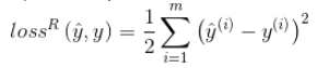
Using the gradient descent method, the gradient is calculated by calculating the derivative of the loss function to the feature (input item), thereby updating the weight. Let m be the number of samples and θ be the weight.

If it is a regression problem, the loss function is generally the mean square error (MSE):

**Therefore, the gradient (derivative) of the loss function of the regression problem to the weight is: **

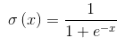
If it is a binary classification problem, the loss function is generally logit loss:

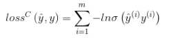
among them,

Represents the step function Sigmoid.

**So the gradient (derivative) of the loss function of the classification problem to the weight is: **

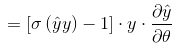
** Correspondingly, the derivatives of the constant term, the first order term, and the cross term respectively** are:

7. Python implementation of FM algorithm

The Python implementation flow chart of the FM algorithm is as follows:

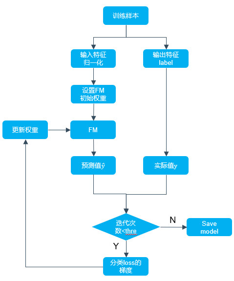
We need to pay attention to the following four points:

1. Initialization parameters, including the initialization of the bias term weight w0, the primary term weight w, and the cross term auxiliary vector;

2. Define the FM algorithm;

3. Definition of the gradient of the loss function;

4. Use gradient descent to update parameters.

The following code snippet is a description of the above four points, where the loss is not the loss of the two classifications, but a part of the gradient of the classification loss:

• loss = self.sigmoid(classLabels[x] * p[0, 0]) -1*

In fact, the gradient of the loss loss of the two categories can be expressed as:

• gradient = (self.sigmoid(classLabels[x] * p[0, 0]) -1)*classLabels[x]p_derivative

Among them, p_derivative represents the derivative of constant term, first order term, and cross term (see Section 6 of this article for details).

FM algorithm code snippet

1   # Initialization parameters
 2   w =zeros((n,1))  #Where n is the number of features
 3   w_0 =0.4         v =normalvariate(0,0.2)*ones((n, k))5for it inrange(self.iter): #Number of iterations
 6    # For each sample, optimize
 7 for x inrange(m):8                 #Pay attention to a mathematical knowledge here: the place corresponding to the dot product usually has a sum, and the place corresponding to the position product is usually not. For details, please refer to the matrix operation rules. The calculation logic here is: http://blog.csdn.net/google19890102/article/details/455327459                 # xi·vi,Matrix dot product of xi and vi
10     inter_1 = dataMatrix[x]* v
11     # The product of the corresponding positions of xi and xi and xi^2 and vi^2 The dot product of the product of the corresponding position
12     inter_2 =multiply(dataMatrix[x], dataMatrix[x])*multiply(v, v)  #multiply multiply corresponding elements
13     # Complete cross-term,xi*vi*xi*vi - xi^2*vi^214                 interaction =sum(multiply(inter_1, inter_1)- inter_2)/2.15                 #Calculate the predicted output
16     p = w_0 + dataMatrix[x]* w + interaction
17 print('classLabels[x]:',classLabels[x])18print('Predicted output p:', p)19                 #Calculate sigmoid(y*pred_y)-1 Accurately speaking, it is not loss. The original author understands that there is a problem here. It is only used as an intermediate parameter to update w. The larger the better, the larger the better, but the following uses gradient descent instead of gradient ascent.
20     loss = self.sigmoid(classLabels[x]* p[0,0])-121if loss >=-1:22                     loss_res ='Positive direction'23else:24                     loss_res ='Opposite direction'25                 #Update parameters
26     w_0 = w_0 - self.alpha * loss * classLabels[x]27for i inrange(n):28if dataMatrix[x, i]!=0:29                         w[i,0]= w[i,0]- self.alpha * loss * classLabels[x]* dataMatrix[x, i]30for j inrange(k):31                             v[i, j]= v[i, j]- self.alpha * loss * classLabels[x]*(32                                     dataMatrix[x, i]* inter_1[0, j]- v[i, j]* dataMatrix[x, i]* dataMatrix[x, i])

Complete implementation of FM algorithm

1 # - *- coding: utf-8-*-23from __future__ import division
 4 from math import exp
 5 from numpy import*6from random import normalvariate  #Normal distribution
 7 from sklearn import preprocessing
 8 import numpy as np
  910'''
 11  data :Data path
 12  feature_potenital :Number of potential decomposition dimensions
 13  alpha: learning rate
 14  iter: number of iterations
 15  _ w,_w_0,_v: weight of the split submatrix
 16  with_col :With columns_name
 17  first_col :Index of the first column of valuable features
 18'''
 192021 classfm(object):22     def __init__(self):23         self.data = None
 24   self.feature_potential = None
 25   self.alpha = None
 26   self.iter = None
 27   self._w = None
 28   self._w_0 = None
 29   self.v = None
 30   self.with_col = None
 31   self.first_col = None
 3233  def min_max(self, data):34         self.data = data
 35   min_max_scaler = preprocessing.MinMaxScaler()36return min_max_scaler.fit_transform(self.data)3738     def loadDataSet(self, data, with_col=True, first_col=2):39         #I’m just idle, pd.read_table()It can be done directly, it seems that the code is very long, and it can be read directly under small data, alas~
 40   self.first_col = first_col
 41   dataMat =[]42         labelMat =[]43         fr =open(data)44         self.with_col = with_col
 45 if self.with_col:46             N =047for line in fr.readlines():48                 # N=Kill the list name at 1
 49 if N >0:50                     currLine = line.strip().split()51                     lineArr =[]52                     featureNum =len(currLine)53for i inrange(self.first_col, featureNum):54                         lineArr.append(float(currLine[i]))55                     dataMat.append(lineArr)56                     labelMat.append(float(currLine[1])*2-1)57                 N = N +158else:59for line in fr.readlines():60                 currLine = line.strip().split()61                 lineArr =[]62                 featureNum =len(currLine)63for i inrange(2, featureNum):64                     lineArr.append(float(currLine[i]))65                 dataMat.append(lineArr)66                 labelMat.append(float(currLine[1])*2-1)67returnmat(self.min_max(dataMat)), labelMat
 6869  def sigmoid(self, inx):70         # return1.0/(1+exp(min(max(-inx,-10),10)))71return1.0/(1+exp(-inx))7273     #Get the corresponding feature weight matrix
 74  def fit(self, data, feature_potential=8, alpha=0.01, iter=100):75         #alpha is the learning rate
 76   self.alpha = alpha
 77   self.feature_potential = feature_potential
 78   self.iter = iter
 79   # dataMatrix uses mat,classLabels is a list
 80   dataMatrix, classLabels = self.loadDataSet(data)81print('dataMatrix:',dataMatrix.shape)82print('classLabels:',classLabels)83         k = self.feature_potential
 84   m, n =shape(dataMatrix)85         #Initialization parameters
 86   w =zeros((n,1))  #Where n is the number of features
 87   w_0 =0.88         v =normalvariate(0,0.2)*ones((n, k))89for it inrange(self.iter): #Number of iterations
 90    # For each sample, optimize
 91 for x inrange(m):92                 #Pay attention to a mathematical knowledge here: the place corresponding to the dot product usually has a sum, and the place corresponding to the position product is usually not. For details, please refer to the matrix operation rules. The calculation logic here is: http://blog.csdn.net/google19890102/article/details/4553274593                 # xi·vi,Matrix dot product of xi and vi
 94     inter_1 = dataMatrix[x]* v
 95     # The product of the corresponding positions of xi and xi and xi^2 and vi^2 The dot product of the product of the corresponding position
 96     inter_2 =multiply(dataMatrix[x], dataMatrix[x])*multiply(v, v)  #multiply multiply corresponding elements
 97     # Complete cross-term,xi*vi*xi*vi - xi^2*vi^298                 interaction =sum(multiply(inter_1, inter_1)- inter_2)/2.99                 #Calculate the predicted output
100     p = w_0 + dataMatrix[x]* w + interaction
101 print('classLabels[x]:',classLabels[x])102print('Predicted output p:', p)103                 #Calculate sigmoid(y*pred_y)-1104                 loss = self.sigmoid(classLabels[x]* p[0,0])-1105if loss >=-1:106                     loss_res ='Positive direction'107else:108                     loss_res ='Opposite direction'109                 #Update parameters
110     w_0 = w_0 - self.alpha * loss * classLabels[x]111for i inrange(n):112if dataMatrix[x, i]!=0:113                         w[i,0]= w[i,0]- self.alpha * loss * classLabels[x]* dataMatrix[x, i]114for j inrange(k):115                             v[i, j]= v[i, j]- self.alpha * loss * classLabels[x]*(116                                     dataMatrix[x, i]* inter_1[0, j]- v[i, j]* dataMatrix[x, i]* dataMatrix[x, i])117print('the no %s times, the loss arrach %s'%(it, loss_res))118         self._w_0, self._w, self._v = w_0, w, v
119120  def predict(self, X):121if(self._w_0 == None)or(self._w == None).any()or(self._v == None).any():122             raise NotFittedError("Estimator not fitted, call `fit` first")123         #Type check
124 ifisinstance(X, np.ndarray):125             pass
126 else:127try:128                 X = np.array(X)129             except:130                 raise TypeError("numpy.ndarray required for X")131         w_0 = self._w_0
132   w = self._w
133   v = self._v
134   m, n =shape(X)135         result =[]136for x inrange(m):137             inter_1 =mat(X[x])* v
138    inter_2 =mat(multiply(X[x], X[x]))*multiply(v, v)  #multiply multiply corresponding elements
139    # Complete cross-term
140    interaction =sum(multiply(inter_1, inter_1)- inter_2)/2.141             p = w_0 + X[x]* w + interaction  #Calculate the predicted output
142    pre = self.sigmoid(p[0,0])143             result.append(pre)144return result
145146  def getAccuracy(self, data):147         dataMatrix, classLabels = self.loadDataSet(data)148         w_0 = self._w_0
149   w = self._w
150   v = self._v
151   m, n =shape(dataMatrix)152         allItem =0153         error =0154         result =[]155for x inrange(m):156             allItem +=1157             inter_1 = dataMatrix[x]* v
158    inter_2 =multiply(dataMatrix[x], dataMatrix[x])*multiply(v, v)  #multiply multiply corresponding elements
159    # Complete cross-term
160    interaction =sum(multiply(inter_1, inter_1)- inter_2)/2.161             p = w_0 + dataMatrix[x]* w + interaction  #Calculate the predicted output
162    pre = self.sigmoid(p[0,0])163             result.append(pre)164if pre <0.5 and classLabels[x]==1.0:165                 error +=1166             elif pre >=0.5 and classLabels[x]==-1.0:167                 error +=1168else:169continue170         # print(result)171         value =1-float(error)/ allItem
172 return value
173174175 classNotFittedError(Exception):176"""
177  Exception classto raise if estimator is used before fitting
178"""
179  pass
180181182 if __name__ =='__main__':183fm()