Python processing PDF and CDF examples

After getting the data, one of the most important tasks is to check the distribution of your data. For the distribution of data, there are two types of pdf and cdf.

The following describes the method of using python to generate pdf:

Use matplotlib's drawing interface hist() to directly draw the pdf distribution;

Using numpy's data processing function histogram(), you can generate pdf distribution data to facilitate subsequent data processing, such as further generation of cdf;

Using seaborn's distplot(), the advantage is that you can fit the pdf distribution and check the distribution type of your own data;

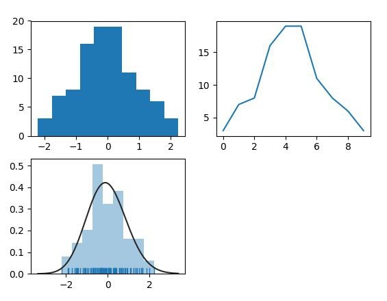
The figure above shows the pdf generated by 3 algorithms. Below is the source code.

from scipy import stats
import matplotlib.pyplot as plt
import numpy as np
import seaborn as sns

arr = np.random.normal(size=100)

# plot histogram
plt.subplot(221)
plt.hist(arr)

# obtain histogram data
plt.subplot(222)
hist, bin_edges = np.histogram(arr)
plt.plot(hist)

# fit histogram curve
plt.subplot(223)
sns.distplot(arr, kde=False, fit=stats.gamma, rug=True)
plt.show()

The following describes how to use python to generate cdf:

Use numpy's data processing function histogram() to generate pdf distribution data, and further generate cdf;

Use seaborn's cumfreq() to draw cdf directly;

The figure above shows the cdf graph generated by two algorithms. Below is the source code.

from scipy import stats
import matplotlib.pyplot as plt
import numpy as np
import seaborn as sns

arr = np.random.normal(size=100)

plt.subplot(121)
hist, bin_edges = np.histogram(arr)
cdf = np.cumsum(hist)
plt.plot(cdf)

plt.subplot(122)
cdf = stats.cumfreq(arr)
plt.plot(cdf[0])

plt.show()

More often, it is necessary to put pdf and cdf together to better display the data distribution. This implementation needs to normalize pdf and cdf respectively.

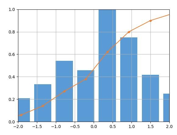
The figure above shows the normalized pdf and cdf. Below is the source code.

from scipy import stats
import matplotlib.pyplot as plt
import numpy as np
import seaborn as sns

arr = np.random.normal(size=100)

hist, bin_edges = np.histogram(arr)
width =(bin_edges[1]- bin_edges[0])*0.8
plt.bar(bin_edges[1:], hist/max(hist), width=width, color='#5B9BD5')

cdf = np.cumsum(hist/sum(hist))
plt.plot(bin_edges[1:], cdf,'-*', color='#ED7D31')

plt.xlim([-2,2])
plt.ylim([0,1])
plt.grid()

plt.show()

The above example of Python processing PDF and CDF is all the content shared by the editor. I hope to give you a reference.