Python one-dimensional two-dimensional interpolation example

One-dimensional interpolation

Interpolation is different from fitting. The interpolation function passes through the sample points, and the fitting function is generally based on the least square method as close as possible to pass through all the sample points. Common interpolation methods include Lagrangian interpolation, segment interpolation, and spline interpolation.

Lagrangian interpolation polynomial: When the number of nodes n is large, the degree of Lagrange interpolation polynomial is higher, inconsistent convergence may occur, and the calculation is complicated. With the increase of sample points, the vibration phenomenon that high-order interpolation will bring errors is called Runge phenomenon.

Piecewise interpolation: Although convergent, the smoothness is poor.

Spline interpolation: Spline interpolation is a form of interpolation using a special piecewise polynomial called spline. Since spline interpolation can use low-order polynomial splines to achieve a smaller interpolation error, which avoids the Runge phenomenon that occurs when using high-order polynomials, spline interpolation has become popular.

View the code piece on CODE and derived from my code piece

#! /usr/bin/env python 
# - *- coding:utf-8-*-import numpy as np 
from scipy import interpolate 
import pylab as pl 
 
x=np.linspace(0,10,11) 
# x=[0.1.2.3.4.5.6.7.8.9.10.] 
y=np.sin(x) 
xnew=np.linspace(0,10,101) 
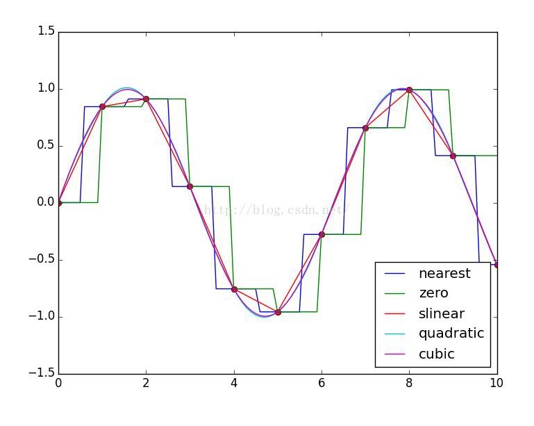
pl.plot(x,y,"ro")for kind in["nearest","zero","slinear","quadratic","cubic"]:#Interpolation method
 #" nearest","zero"Interpolate for steps
 # slinear linear interpolation
 #" quadratic","cubic"Interpolate for 2nd and 3rd B-spline curves
 f=interpolate.interp1d(x,y,kind=kind) 
 # ‘slinear', ‘quadratic' and ‘cubic' refer to a spline interpolation of first, second or third order) 
 ynew=f(xnew) 
 pl.plot(xnew,ynew,label=str(kind)) 
pl.legend(loc="lower right") 
pl.show()

result:

Two-dimensional interpolation

The method is similar to one-dimensional data interpolation, which is two-dimensional spline interpolation.

View the code piece on CODE and derived from my code piece

# - *- coding: utf-8-*-""" 
Demonstrate two-dimensional interpolation.
""" 
import numpy as np 
from scipy import interpolate 
import pylab as pl 
import matplotlib as mpl 
 
def func(x, y):return(x+y)*np.exp(-5.0*(x**2+ y**2)) 
 
# X-Y axis is divided into 15*15 grid
y,x= np.mgrid[-1:1:15j,-1:1:15j] 
 
fvals =func(x,y) #Calculate the function value at each grid point 15*Value of 15
print len(fvals[0]) 
 
# Cubic spline two-dimensional interpolation
newfunc = interpolate.interp2d(x, y, fvals, kind='cubic') 
 
# Calculate 100*Interpolation on a grid of 100
xnew = np.linspace(-1,1,100)#x 
ynew = np.linspace(-1,1,100)#y 
fnew =newfunc(xnew, ynew)#Just y value 100*Value of 100
 
# Drawing
# In order to compare the difference before and after interpolation more clearly, use the keyword parameter interpolation='nearest' 
# Close imshow()Built-in interpolation operation.
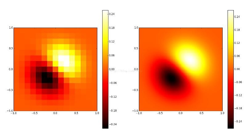
pl.subplot(121) 
im1=pl.imshow(fvals, extent=[-1,1,-1,1], cmap=mpl.cm.hot, interpolation='nearest', origin="lower")#pl.cm.jet 
# extent=[-1,1,-1,1]X,y range favals are
pl.colorbar(im1) 
 
pl.subplot(122) 
im2=pl.imshow(fnew, extent=[-1,1,-1,1], cmap=mpl.cm.hot, interpolation='nearest', origin="lower") 
pl.colorbar(im2) 
 
pl.show()

The left picture is the original data, and the right picture is the result of two-dimensional interpolation.

3D display method of 2D interpolation

View the code piece on CODE and derived from my code piece

# - *- coding: utf-8-*-""" 
Demonstrate two-dimensional interpolation.
""" 
# - *- coding: utf-8-*-import numpy as np 
from mpl_toolkits.mplot3d import Axes3D 
import matplotlib as mpl 
from scipy import interpolate 
import matplotlib.cm as cm 
import matplotlib.pyplot as plt 
 
def func(x, y):return(x+y)*np.exp(-5.0*(x**2+ y**2)) 
 
# X-Y axis is divided into 20*20 grid
x = np.linspace(-1,1,20) 
y = np.linspace(-1,1,20) 
x, y = np.meshgrid(x, y)#20*20 grid data
 
fvals =func(x,y) #Calculate the function value at each grid point 15*Value of 15
 
fig = plt.figure(figsize=(9,6)) 
# Draw sub-graph1 
ax=plt.subplot(1,2,1,projection ='3d') 
surf = ax.plot_surface(x, y, fvals, rstride=2, cstride=2, cmap=cm.coolwarm,linewidth=0.5, antialiased=True) 
ax.set_xlabel('x') 
ax.set_ylabel('y') 
ax.set_zlabel('f(x, y)') 
plt.colorbar(surf, shrink=0.5, aspect=5)#Label
 
# Two-dimensional interpolation
newfunc = interpolate.interp2d(x, y, fvals, kind='cubic')#newfunc is a function
 
# Calculate 100*Interpolation on a grid of 100
xnew = np.linspace(-1,1,100)#x 
ynew = np.linspace(-1,1,100)#y 
fnew =newfunc(xnew, ynew)#Just y value 100*Value of 100 np.shape(fnew) is 100*100 
xnew, ynew = np.meshgrid(xnew, ynew) 
ax2=plt.subplot(1,2,2,projection ='3d') 
surf2 = ax2.plot_surface(xnew, ynew, fnew, rstride=2, cstride=2, cmap=cm.coolwarm,linewidth=0.5, antialiased=True) 
ax2.set_xlabel('xnew') 
ax2.set_ylabel('ynew') 
ax2.set_zlabel('fnew(x, y)') 
plt.colorbar(surf2, shrink=0.5, aspect=5)#Label
 
plt.show()

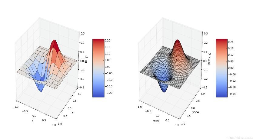
The function value of the two-dimensional data set on the left will appear rough due to fewer samples. The figure on the right performs cubic spline interpolation on the two-dimensional sample data, and the sample value of more data points is obtained by fitting, and the image is obviously smoother after drawing.

Supplementary knowledge: implementation method of dataframe two-dimensional lookup table interpolation in python

Today, when calculating the power of wind turbines to capture wind energy, it is necessary to make a power efficiency reduction of the wind energy within the sweeping area of the blade, that is, the Cp coefficient. Cp is defined as follows, that is, the ratio of the actual used wind energy to the input wind energy

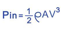
The input wind energy is a function of air density and wind speed, which can be directly calculated:

Then the actual ability obtained is the product of Pin and Cp.

Cp is usually a two-dimensional table, the abscissa is TSR (the ratio of blade tip speed to wind speed), and the ordinate is PITCH Angle (blade angle). The operating data of the wind turbine contains wind speed, rotational speed and blade angle information, and by directly reading into the DataFrame, then it is necessary to look up the Cp table based on the TSR and PA and interpolate to obtain the Cp. Scipy.interpolate.interp2d is mainly used to create an interpolation function and look up the table. In addition, the interpolation function cannot be used directly in the Dataframe. Here, a for loop branch interpolation look up table is made.

from scipy.interpolate import interp2d
df_rotormap = pd.read_csv('filepath',header = None) #Read Cp table
x = np.array(df_rotormap.iloc[:,0].dropna()) #The X coordinate of the Cp table is TSR
y = np.array(df_rotormap.iloc[:,1]) #The Y coordinate of the Cp table is pitch angle
z = np.array(df_rotormap.iloc[:,2:]) #The specific value of Cp table, y row x column

rho =1.225 #kg/m3
s =(141/2)**2*np.pi #m2
df_cal['TSR']= df_cal['Generator speed (PDM1)']/148*141*np.pi/60/df_cal['Wind speed']

func_new =interp2d(x,y,z,kind ='linear') #Define two-dimensional table interpolation function, select linear interpolation

cp_list =[]for i inrange(df_cal.shape[0]):
 cp =float(func_new(df_cal['TSR'][i],df_cal['No. 1 blade angle'][i])) #Enter X,Y coordinate, output Cp calculated by interpolation
 cp_list.append(cp)

df_cal['cp']= cp_list #Put Cp back into the Dataframe

df_cal['air_power']=0.5*rho*s*df_cal['Wind speed']**3*df_cal['cp']

The above python one-dimensional two-dimensional interpolation example is all the content shared by the editor, I hope to give you a reference.