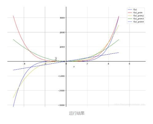
Example of python calculating derivative and plotting
I will stop talking nonsense, just go to the code!
import math
import numpy as np
import matplotlib.pyplot as plt
from sympy import* #Used for scientific calculations such as derivative integral


def dif(left,right,step):#Derivative left and right interval and interval
 x,y =symbols('x y')#Introduce xy variables
 expr =pow(x,5)#Calculation expression
 x_value =[] #save x value
 y_value =[] #save x f(x) value
 y_value_dif =[] #save x f(x)_dot value
 y_value_dif2 =[] #save x f(x)_dot2 value
 y_value_dif3 =[] #save x f(x)_dot3 value
 y_value_dif4 =[] #save x f(x)_dot4 value
 # print(expand(exp(I*x), complex=True))#Expand the complex exponent into the form of real and imaginary parts
 expr_dif =diff(expr,x,1)
 expr_dif2 =diff(expr,x,2)
 expr_dif3 =diff(expr,x,3)
 expr_dif4 =diff(expr,x,4)for i in np.arange(left,right,step):
 x_value.append(i)
 y_value.append(expr.subs('x',i))#Substitute the value of i into the expression
 y_value_dif.append(expr_dif.subs('x',i))#Substitute the value of i into the derivative expression
 y_value_dif2.append(expr_dif2.subs('x',i))#Substitute the value of i into the second-order derivative expression
 y_value_dif3.append(expr_dif3.subs('x',i))#Substitute the value of i into the third-order derivative expression
 y_value_dif4.append(expr_dif4.subs('x',i))#Substitute the value of i into the fourth-order derivative expression
 draw_plot_set()#Set drawing format
 plt.plot(x_value,y_value,"b-",linewidth=1,label='f(x)='+str(expr)) #Drawing
 plt.plot(x_value,y_value_dif,"r-",linewidth=1,label='f(x)_prim') #Drawing
 plt.plot(x_value,y_value_dif2,"y-",linewidth=1,label='f(x)_prim2') #Drawing
 plt.plot(x_value,y_value_dif3,"g-",linewidth=1,label='f(x)_prim3') #Drawing
 plt.plot(x_value,y_value_dif4,"b-",linewidth=1,label='f(x)_prim4') #Drawing

 plt.legend()#Show legend
 plt.show()#Display image


def draw_plot_set():#Set drawing format
 plt.figure()
 ax = plt.gca()
 # Change axis position
 ax.spines['right'].set_color('none')#Delete original axis
 ax.spines['top'].set_color('none')#Delete original axis
 ax.xaxis.set_ticks_position('bottom')#Add axis at 0
 ax.spines['bottom'].set_position(('data',0))
 ax.yaxis.set_ticks_position('left')#Add axis at 0
 ax.spines['left'].set_position(('data',0))
 # Set coordinate name
 plt.ylabel('f(x)')
 plt.xlabel('x')

 plt.grid(True)#Open grid


if __name__ =='__main__':dif(-5,5,0.01)

Supplementary extension: python uses the sympy library to derive a function, and the numpy library uses the program to calculate the derivation result
In the process of python data processing, we often encounter such a situation. It is necessary to obtain a partial derivative of a function expression and substitute specific values into the derivative formula.
The function that can usually be used to derive function in python is the diff() function in the sympy library.
But the derivative he usually finds is just a symbolic expression. It cannot be directly brought into data use.
The following example:
import sympy as sp
import numpy as np
x,y = sp.symbols('x y')
z = sp.sin(2*sp.pi*x+2*y/5)
zx = sp.diff(z,x)
zy = sp.diff(z,y)print(zx)print(zy)
The output is:
2* pi*cos(2*pi*x +2*y/5)2*cos(2*pi*x +2*y/5)/5
**So how to solve this problem? **
After using the evalf() function to assign values to x and y respectively, and then use float for type conversion, then numpy can be used for numerical calculation.
The following example:
import sympy as sp
import numpy as np
x,y = sp.symbols('x y')
z = sp.sin(2*sp.pi*x+2*y/5)
zx = sp.diff(z,x)
zy = sp.diff(z,y)
x1 =10
y1 =5
z_x1 =float(zx.evalf(subs={x:x1,y:y1}))
z_y1 =float(zy.evalf(subs={x:x1,y:y1}))print(z_x1)print(z_y1)
The output result:
-2.61472768902227-0.16645873461885696
What if my x or y is not a single value? It is an array.
We can use a loop to complete.
The following example:
import sympy as sp
import numpy as np
x,y = sp.symbols('x y')
z = sp.sin(2*sp.pi*x+2*y/5)
zx = sp.diff(z,x)
zy = sp.diff(z,y)
x_array = np.linspace(-5,5,10)
y_array = np.linspace(-5,5,10)
temp_x =[]#First define an empty list for storing the partial derivative of x
temp_y =[]#First define an empty list for storing y partial derivatives
for i inrange(10):
 z_x =float(zx.evalf(subs={x:x_array[i],y:y_array[i]}))
 temp_x.append(z_x)#Add the calculated partial derivatives to the list one by one
 z_y =float(zy.evalf(subs={x:x_array[i],y:y_array[i]}))
 temp_y.append(z_y)
zx_array = np.array(temp_x)#Convert list to array
zy_array = np.array(temp_y)print(zx_array)print(zy_array)
The output is:
[-2.614727694.111638646.029462890.89585862-5.2854481-5.28544810.895858626.029462894.11163864-2.61472769][-0.166458730.261755050.383847530.05703213-0.33648208-0.336482080.057032130.383847530.26175505-0.16645873]
In this way, the derivation result obtained by sympy is realized, and the numerical calculation is performed in the numpy library.
The above example of python calculating derivative and drawing is all the content shared by the editor, I hope to give you a reference.
Recommended Posts