Python Data Science: Chi-Square Test
The variable analysis introduced before:
① Correlation analysis: The relationship between a continuous variable and a continuous variable.
② Two-sample t-test: the relationship between a dichotomous categorical variable and a continuous variable.
③ Analysis of variance: The relationship between a multi-categorical categorical variable and a continuous variable.
This introduction:
Chi-square test: the relationship between a dichotomous categorical variable or a multi-class categorical variable and a dichotomous categorical variable.
If the distribution of one of the variables changes with the level of the other variable, then the two categorical variables are related.
The chi-square test cannot show the strength of the correlation between two categorical variables, but can only show whether the two categorical variables are related.
/ 01 / Data mining technology and methods
Data mining methods are divided into two types: descriptive and predictive.
Both methods are based on historical data for analysis.
Descriptive models are used to directly reflect historical conditions and provide inspiration for subsequent analysis.
Predictive models find patterns from historical data and use them to predict the future.
Common algorithms for descriptive data mining: cluster analysis, association rule analysis.
Commonly used algorithms for predictive data mining: linear regression, logistic regression, neural network, decision tree, support vector machine.
/ 02 / Chi-square test
01 Contingency table
The contingency table is a category summary table.
Set each category of one of the two categorical variables to be analyzed as a column variable.
Each category of the other variable is set as a row variable, and the middle corresponds to the frequency under different categories.
Let's take the data in the book as an example to explore the relationship between whether a categorical variable is in default and whether a categorical variable is bankrupt.
The data used can be obtained by reading the original text.
import pandas as pd

df = pd.read_csv('accepts.csv')
# crosstab:Cross table,margins:Show sum
cross_table = pd.crosstab(df['bankruptcy_ind'], df['bad_ind'], margins=True)print(cross_table)
Output the result.

It's not easy to judge the relationship here, and the following is converted to frequency.
# div:Convert list to frequency data
cross_table_last = cross_table.div(cross_table['All'], axis=0)print(cross_table_last)
Output the result.

It can be seen that the difference is not very large, but we cannot directly draw conclusions.
It can only be said that there is a greater possibility, whether bankruptcy is not related to whether or not a breach of contract.
Next, the chi-square test is used to determine the conclusion and make it statistically significant.
02 Chi-square test
Chi-square test is to compare the degree of agreement between the expected frequency and the actual frequency.
The actual frequency is the actual number of observations in the cell, and the denominator of the actual frequency is the total number of samples.
The expected frequency is the frequency when the variables are independent of each other, calculated by the expected frequency, and the expected frequency is derived from the actual frequency.
The null hypothesis of the chi-square test is that the expected frequency is equal to the actual frequency, that is, the two categorical variables are irrelevant, and the alternative hypothesis is related.
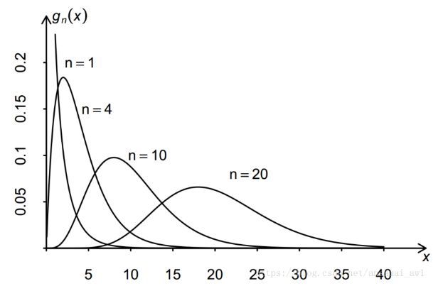
The chi-square statistic is calculated by formula, and its value obeys the chi-square distribution.
The chi-square distribution diagram is as follows, the horizontal axis is the chi-square statistic value, the vertical axis is the P value, and n is the degree of freedom.

In this case, I personally think that the degree of freedom should be 1. I wonder why the book says that the degree of freedom is 2? ? ?
Let's use Python to perform a chi-square test on the data.
from scipy import stats

# chi2_contingency:Chi-square test,chisq:Chi-square statistic value,expected_freq:Expected frequency
print('chisq = %6.4f\n p-value = %6.4f\n dof = %i\n expected_freq = %s'%stats.chi2_contingency(cross_table))
Output the result.

The chi-square value is 2.9167, the P value is 0.5719, and the significance level is 0.05, indicating that there is no reason to reject the null hypothesis.
That is, the two categorical variables are irrelevant, and whether there is a breach of contract has nothing to do with whether it is bankrupt.
/ 03 / Summary
Here is a summary of the knowledge about degrees of freedom.
As a mechanic, there should be only 6 degrees of freedom for me.
Three rotations and three movements, for X, Y, Z axis.
But this is not the case in statistics.
①The degree of freedom refers to the number of independent or freely variable data in the sample when the overall parameter is estimated by the statistical quantity of the sample.
② The degree of freedom is the number of data that can be changed independently. As long as the number of n-1 is determined, the number of n is determined, and it cannot be changed freely.
To be honest, it's still a bit dizzy...
Recommended Posts