Python Data Science: Linear Regression Diagnosis
Following the previous linear regression article, the portal is as follows.
[ Python Data Science: Linear Regression](http://mp.weixin.qq.com/s?__biz=MzU4OTYzNjE2OQ==&mid=2247484227&idx=1&sn=4e383b99c85c46841cc65c4f5b298d30&chksm=fdcb3465cabc85e
Prerequisites for multiple linear regression:
- The dependent variable cannot have a linear relationship with the disturbance term
- There must be a linear relationship between the independent variable and the dependent variable
- There can be no too strong linear relationship between the independent variables
- Disturbance terms or residuals are independent and should follow a normal distribution with a mean of 0 and a certain variance
/ 01 / Residual Error Analysis
Residual error analysis is an important part of linear regression diagnosis.
There are three prerequisites for the residuals to obey:
- Homogeneity of residual variance
- Residuals are independent and identically distributed
- Residuals cannot be correlated with independent variables (cannot be tested)
View the residuals by viewing the residual graph.
Residual graphs can be divided into four categories:
- The residuals are normally distributed: the residuals are randomly distributed, the upper and lower bounds are basically symmetrical, there is no obvious autocorrelation, and the variances are basically homogeneous
- The residual curve distribution: the residual and the predicted value are in a curve relationship, indicating that the independent variable and the dependent variable are not linear
- Uneven residual variance: the upper and lower bounds of the residual are basically symmetrical, but as the predicted value increases, the upper and lower ranges will also increase
- Periodic change of residual error: The residual error changes periodically with the increase of the predicted value, indicating that the independent variable and the dependent variable may change periodically
Let's take the model in the previous linear regression article as an example.
# Simple linear regression model,Average expenditure and income
ana1 = lm_s
# The predicted value of the training data set
exp['Pred']= ana1.predict(exp)
# Residuals of the training data set
exp['resid']= ana1.resid
# Draw a scatter plot of income and residuals
exp.plot('Income','resid', kind='scatter')
plt.show()
The residuals of the model are obtained. As the predicted value increases, the residuals basically remain symmetrical.
However, the magnitude of the positive and negative residuals tends to gradually become larger, that is, the model has the problem of uneven variance.
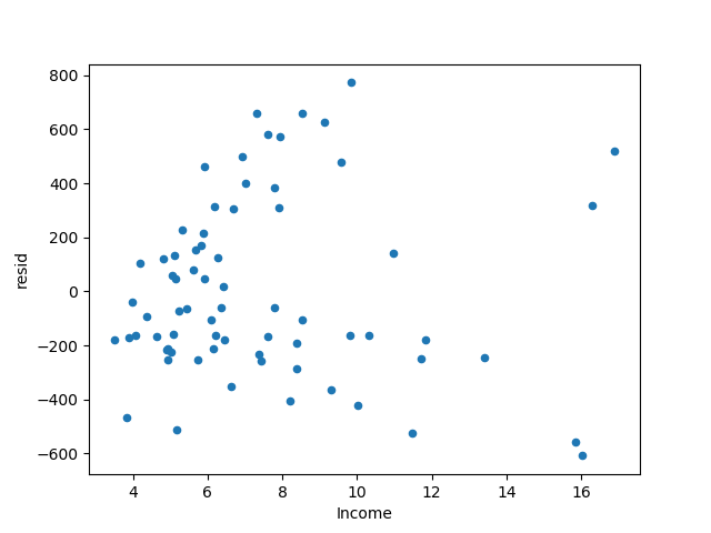
The processing method of heteroscedasticity can take the data in logarithm, so here the average expenditure data is processed in logarithm.
# Use simple linear regression to build a model,Log average expenditure data
ana2 =ols('avg_exp_ln ~ Income', data=exp).fit()
exp['Pred']= ana2.predict(exp)
# Residuals of the training data set
exp['resid']= ana2.resid
# Draw a scatter plot of income and residuals
exp.plot('Income','resid', kind='scatter')
plt.show()
Obtain the residuals of the model, and find that the magnitude of the positive and negative residuals has a trend of improvement.
The book says that the heteroscedasticity phenomenon has been improved, but I feel it's pretty good...
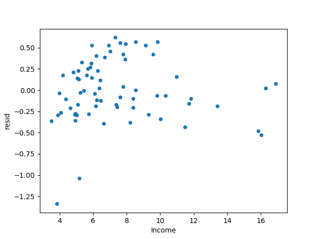
The above only takes the logarithm for the average expenditure data, and the following also takes the logarithm for the income data, making the percentage increase of the two roughly the same.
# Logarithm of income data,np.log(e)=1
exp['Income_ln']= np.log(exp['Income'])
# Use simple linear regression to build a model,Log average expenditure data
ana3 =ols('avg_exp_ln ~ Income_ln', data=exp).fit()
exp['Pred']= ana3.predict(exp)
# Residuals of the training data set
exp['resid']= ana3.resid
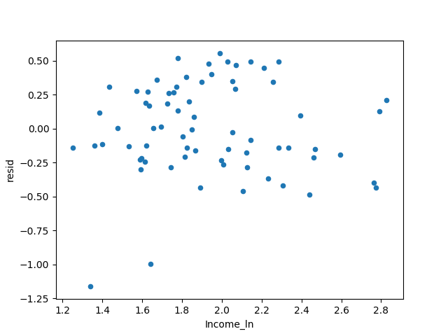
# Draw a scatter plot of income and residuals
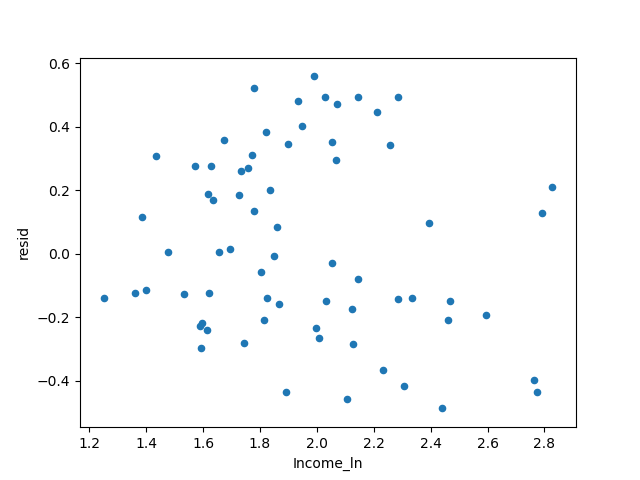
exp.plot('Income_ln','resid', kind='scatter')
plt.show()
The book says that the heteroscedasticity phenomenon is eliminated. I really don’t see any big difference from the previous picture...
Compare the R² situation of the three models.
# Get the R² value of the three models
r_sq ={'exp~Income': ana1.rsquared,'ln(exp)~Income': ana2.rsquared,'ln(exp)~ln(Income)': ana3.rsquared}print(r_sq)
# Output result
{' ln(exp)~Income':0.4030855555329649,'ln(exp)~ln(Income)':0.480392799389311,'exp~Income':0.45429062315565294}
It is found that the R² of the logarithmic model is the largest, and the model is considered the best of the three.
DW test (Durbin-Watson test) can be used to judge the autocorrelation relationship of residuals.
When the DW value approaches 2, it can be considered that the residual has no autocorrelation relationship.
The following are the judgment indicators output by the model with all logarithms.
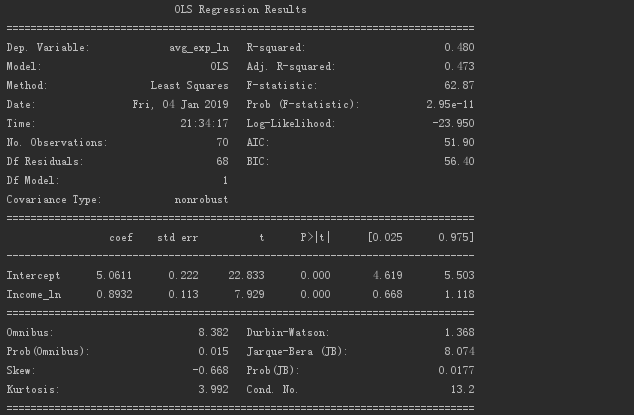
It is found that all models that take logarithms have a DW value of 1.368.
I don’t know what the correlation is, it may be a positive correlation...
/ 02/ Strong influence points
When a point is too far away from the group, the fitted regression line will be strongly disturbed by this point, thereby changing the position of the regression line.
This is the point of strong influence.
Here we can use the predicted value-studentized residual map to identify strong influence points.
Studentized residual (SR) refers to the standardized residual.
# Studentized residual calculation
exp['resid_t']=(exp['resid']- exp['resid'].mean())/ exp['resid'].std()
# Take 2 when the sample size is a few hundred,Take 3prints when the sample size is thousands(exp[abs(exp['resid_t'])>2])
The output is as follows.

There are two in total. From the previous scatter plot, everyone should be able to know which two points are.
The regression model is established based on the data that removes strong influence points.
# Use simple linear regression to build a model,Remove strong points of influence
exp2 = exp[abs(exp['resid_t'])<=2].copy()
ana4 =ols('avg_exp_ln ~ Income_ln', data=exp2).fit()
exp2['Pred']= ana3.predict(exp)
# Residuals of the training data set
exp2['resid']= ana3.resid
# Draw a scatter plot of income and residuals
exp2.plot('Income_ln','resid', kind='scatter')
plt.show()
got the answer.
This residual result is still good.
/ 03 / Multicollinearity analysis
There can be no strong collinearity between the independent variables, also known as multicollinearity.
This time, the variance inflation factor is used to diagnose and reduce multicollinearity.
In the previous data, add local average house price and local average income data.
exp2['dist_home_val_ln']= np.log(exp['dist_home_val'])
exp2['dist_avg_income_ln']= np.log(exp['dist_avg_income'])

def vif(df, col_i):
 # Get variables
 cols =list(df.columns)
 # Remove dependent variables
 cols.remove(col_i)
 # Get argument
 cols_noti = cols
 # Multivariate linear regression model establishment and acquisition model R²
 formula = col_i +'~'+'+'.join(cols_noti)
 r2 =ols(formula, df).fit().rsquared
 # Calculate the variance inflation factor
 return1./(1.- r2)

# Get independent variable data
exog = exp2[['Age','Income_ln','dist_home_val_ln','dist_avg_income_ln']]
# Iterate over the arguments,Get its VIF value
for i in exog.columns:print(i,'\t',vif(df=exog, col_i=i))
The result obtained.
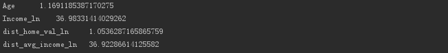
It is found that the variance inflation factor between income and local average income is greater than 10, indicating that there is multicollinearity.
It stands to reason that one of the variables should be deleted at this time.
The ratio of higher average income is used here instead of the income data column, which can better reflect the information.
# Percentage higher than average income
exp2['high_avg_ratio']= exp['high_avg']/ exp2['dist_avg_income']
# Get independent variable data
exog2 = exp2[['Age','high_avg_ratio','dist_home_val_ln','dist_avg_income_ln']]
# Iterate over the arguments,Get its VIF value
for i in exog2.columns:print(i,'\t',vif(df=exog2, col_i=i))
Output the result.
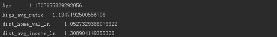
It is found that the variance expansion factor of each variable is small, indicating that there is no collinearity.
Of course, the above methods can only reduce the interference of collinearity on the model, but cannot completely eliminate multicollinearity.
/ 04 / Summary
The steps to build a reasonable linear regression model are as follows.
Initial analysis: Determine research objectives and collect data.
Variable selection: Find the independent variable that has an influence on the dependent variable.
Validation model assumptions:
- Set up the model, select the regression method, select the variables, and in what form the variables are put into the model
- The explanatory variable and the disturbance term cannot be correlated
- There must be no strong linear relationship between explanatory variables
- Disturbance terms are independent and identically distributed
- Disturbance items obey normal distribution
Diagnosis and analysis of multicollinearity and strong influence points: modified regression model.
Prediction and interpretation: use models to predict and explain.
To be honest, this part is not easy to understand.
Most of the time I choose Mark first, and then slowly digest...
Recommended Posts