Python Data Science: Logistic Regression
It's been a long time since I wrote the content of data mining, so I will continue to talk about this issue.
Learn about logistic regression models.

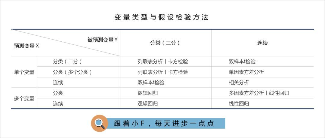
From the above figure, we can see that the logistic regression model is mostly used when the dependent variable is a categorical variable.
Therefore, for this data prediction, a two-category variable (whether default) is also selected.
/ 01 / Logistic regression
Logistic regression transforms the value range of the linear equation with positive or negative infinity through logit conversion to (0, 1), which is exactly the same as the value range of probability.
The specific formulas are not listed, so I will stop here.
If you want to know more, you can consult related materials or books.
Logistic regression is to construct a logit transformation to make probability prediction.
Linear regression is also a predictive method.
But Logistic regression is suitable for predicting categorical variables, and it predicts the probability of an interval from 0 to 1.
Linear regression is suitable for predicting continuous variables.
In addition, if multiple target variables are encountered, Logistic regression can also predict.
But more often, analysts are more inclined to integrate multiple target variables into binary target variables based on business understanding, and then perform Logistic regression (if feasible).
Logistic regression predicts the probability of an event, and uses maximum likelihood estimation to estimate the parameters of the probability.
/ 02/ Python implementation
Convention, continue to use the data provided in the book.
A dataset of car default loans.
The variables involved are default'', has been bankruptcy mark'', number of bad credit events in five years'', longest account duration'', recyclable loan account usage ratio'', FICO score'', ``loan amount/recommended selling price*100 ""driven distance".
Read the data and sample the data. The ratio of training set to test set is 7:3.
import numpy as np
import pandas as pd
import statsmodels.api as sm
import matplotlib.pyplot as plt
import sklearn.metrics as metrics
import statsmodels.formula.api as smf

# Eliminate pandas output ellipsis
pd.set_option('display.max_columns', None)
# Read data,skipinitialspace:Ignore white space after delimiter
accepts = pd.read_csv('accepts.csv', skipinitialspace=True)
# dropna:Delete missing data
accepts = accepts.dropna(axis=0, how='any')
# Frac sampling ratio,For 70%
train = accepts.sample(frac=0.7, random_state=1234).copy()
test = accepts[~ accepts.index.isin(train.index)].copy()print('Training set sample size: %i \n Test set sample size: %i'%(len(train),len(test)))
After some practice, I found that different extraction ratios will lead to different final results.
In addition, the above uses random sampling, and the default ratios in the training set and the test set will be different.
So you can also consider stratified sampling to ensure a fixed proportion of samples.
Next, generalized linear regression is used, and logit transformation is specified to process the data.
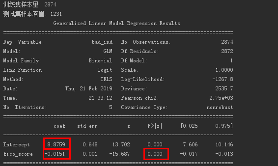
lg = smf.glm('bad_ind ~ fico_score', data=train, family=sm.families.Binomial(sm.families.links.logit)).fit()print(lg.summary())
Logistic regression result obtained for FICO score.

Get the coefficient and intercept of the regression equation.
The value of e to the -0.0151 power is about 0.985.
This means that every time the FICO score increases by one unit, the probability of default is 0.985 times the original, and the probability of default decreases.
The realization of multiple logistic regression is as follows.
formula ="""bad_ind ~ fico_score + bankruptcy_ind + tot_derog + age_oldest_tr + rev_util + ltv + veh_mileage"""
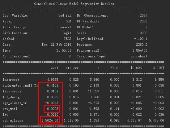
lg_m = smf.glm(formula=formula, data=train, family=sm.families.Binomial(sm.families.links.logit)).fit()print(lg_m.summary())
The logistic regression results obtained are as follows.

Obtain the coefficients of each variable. Among them, the coefficients of the two variables of "recycling loan account usage ratio" and "mileage traveled" are relatively insignificant and can be deleted.
Of course, it can also be combined with the forward method used in linear regression to filter variables based on the AIC criterion.
# Forward regression
def forward_select(data, response):"""data is data containing independent variables and dependent variables,response is the dependent variable"""
 # Get list of arguments
 remaining =set(data.columns)
 remaining.remove(response)
 selected =[]
 # Define data type(Positive infinity)
 current_score, best_new_score =float('inf'),float('inf')
 # When the argument list contains arguments
 while remaining:
  aic_with_candidates =[]
  # Loop through the list of arguments
  for candidates in remaining:
   # Build expression,The independent variable will continue to increase
   formula ="{} ~ {}".format(response,' + '.join(selected +[candidates]))
   # AIC interpretation strength of the independent variable generated
   aic = smf.glm(formula=formula, data=data, family=sm.families.Binomial(sm.families.links.logit)).fit().aic
   # Get the AIC explanation strength list of the independent variable
   aic_with_candidates.append((aic, candidates))
  # Sort the interpretation strength list from largest to smallest
  aic_with_candidates.sort(reverse=True)
  # Get the maximum explained strength(Minimum AIC value)And independent variables
  best_new_score, best_candidate = aic_with_candidates.pop()
  # 1. Positive infinity is greater than the maximum explanatory power 2.The AIC value of the previous experiment must be greater than that of the next experiment,That is, the more variables you add,The AIC value should be smaller,The better the model
  if current_score > best_new_score:
   # Remove the most influential independent variables
   remaining.remove(best_candidate)
   # Add influential independent variables
   selected.append(best_candidate)
   # Assign the AIC value of this experiment
   current_score = best_new_score
   print('aic is {},continue!'.format(current_score))else:print('forward selection over!')break
 # Use a list of influential independent variables,Perform linear regression on the data
 formula ="{} ~ {}".format(response,' + '.join(selected))print('final formula is {}'.format(formula))
 model = smf.glm(formula=formula, data=data, family=sm.families.Binomial(sm.families.links.logit)).fit()return model

# Use forward regression to filter variables,Use the selected variables to build a regression model
data_for_select = train[['bad_ind','fico_score','bankruptcy_ind','tot_derog','age_oldest_tr','rev_util','ltv','veh_mileage']]
lg_m1 =forward_select(data=data_for_select, response='bad_ind')print(lg_m1.summary())
The output is as follows.

It was found that the variables were not filtered out.
But observing the two variables mentioned earlier, their changes to the AIC value are minimal.
Although the AIC value has been reduced, it can be deleted based on the changes.
This is different from the book...
Next, use the variance expansion factor calculation function in linear regression to complete the multicollinearity judgment of the independent variables in logistic regression.
def vif(df, col_i):
 # Get variables
 cols =list(df.columns)
 # Remove dependent variables
 cols.remove(col_i)
 # Get argument
 cols_noti = cols
 # Multivariate linear regression model establishment and acquisition model R²
 formula = col_i +'~'+'+'.join(cols_noti)
 r2 = smf.ols(formula, df).fit().rsquared
 # Calculate the variance expansion coefficient
 return1./(1.- r2)

# Get independent variable data
exog = train[['fico_score','tot_derog','age_oldest_tr','rev_util','ltv','veh_mileage']]
# Iterate over the arguments,Get its VIF value
for i in exog.columns:print(i,'\t',vif(df=exog, col_i=i))
The output is as follows.

It is found that all are less than the threshold of 10, indicating that the independent variables have no significant multicollinearity.
Next, use the trained model to predict the test.
train['proba']= lg_m1.predict(train)
test['proba']= lg_m1.predict(test)print(test['proba'].head())
# Greater than 0.5 for default
test['prediction']=(test['proba']>0.5).astype('int')
# print(test['prediction'])
The output is as follows.

/ 03 / Model evaluation
Logistic regression models are mostly used as ranking models.
The indicators for evaluating the ranking model include ROC curve, KS statistics, Lorentz curve and so on.
This time it is illustrated by ROC curve.
ROC curve, also known as receiver operating characteristic curve, is used to describe the model's resolving power. The higher the graph above the diagonal, the better the model.
In the ROC curve, it mainly involves two indexes of sensitivity and specificity.
Sensitivity indicates how well the model predicts the response.
Specificity indicates the degree of coverage that the model predicts not to respond.
Coverage indicates the proportion of actual observations that are accurately predicted.
The ROC curve is a scatter curve graph with specificity as the X axis and sensitivity as the Y axis.
The steeper the ROC curve, the stronger the coverage of the response in the observations with high prediction probability, and the less falsely reported responses, indicating the better the model effect.
Finally, the AUC value (the area under the curve) can be used to judge the quality of the model.
"0.5, 0.7"-the effect is low, "0.7, 0.85"-the effect is average, "0.85, 0.95"-the effect is good, "0.95, 1"-the effect is very good.
The implementation code of ROC curve in this example is as follows.
acc =sum(test['prediction']== test['bad_ind'])/ np.float(len(test))
# Forecast model accuracy
print('The accurancy is %.2f'% acc)
# Output 0.Cross summary table at 5 threshold
print(pd.crosstab(test.bad_ind, test.prediction, margins=True))for i in np.arange(0,1,0.1):
 prediction =(test['proba']> i).astype('int')
 confusion_matrix = pd.crosstab(test.bad_ind, prediction, margins=True)
 precision = confusion_matrix.ix[1,1]/ confusion_matrix.ix['All',1]
 recall = confusion_matrix.ix[1,1]/ confusion_matrix.ix[1,'All']
 f1_score =2*(precision * recall)/(precision + recall)print('threshold: %s, precision: %.2f, recall: %.2f, f1_score: %.2f'%(i, precision, recall, f1_score))

# Draw ROC curve
fpr_test, tpr_test, th_test = metrics.roc_curve(test.bad_ind, test.proba)
fpr_train, tpr_train, th_train = metrics.roc_curve(train.bad_ind, train.proba)
plt.figure(figsize=[3,3])
plt.plot(fpr_test, tpr_test,'b--')
plt.plot(fpr_train, tpr_train,'r-')
plt.title('ROC curve')
plt.show()

# Calculate AUC value
print('AUC = %.4f'% metrics.auc(fpr_train, tpr_train))print(metrics.auc(fpr_train, tpr_train))
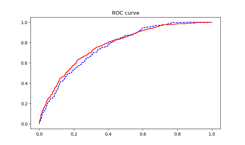
The output ROC curve is as follows.

The accuracy output of the prediction model is 0.81.
The output AUC value is 0.7732, the model effect is average.
Recommended Posts