Python Data Science: Linear Regression
The variable analysis introduced before:
① Correlation analysis: The relationship between a continuous variable and a continuous variable.
② Two-sample t-test: the relationship between a dichotomous categorical variable and a continuous variable.
③ Analysis of variance: The relationship between a multi-categorical categorical variable and a continuous variable.
④ Chi-square test: the relationship between a dichotomous categorical variable or multi-class categorical variable and a dichotomous categorical variable.
This introduction:
Linear regression: The relationship between multiple continuous variables and one continuous variable.
Among them, linear regression is divided into simple linear regression and multiple linear regression.
/ 01 / Data Analysis and Data Mining
Database: A tool for storing data. Because Python is a memory calculation, it is difficult to process dozens of gigabytes of data, so sometimes data cleaning needs to be performed in the database.
Statistics: Data analysis methods for small data, such as data sampling, descriptive analysis, and result testing.
Artificial Intelligence/Machine Learning/Pattern Recognition: Neural network algorithms, imitating the operation of the human nervous system, can not only learn from training data, but also predict unknown data based on the results of learning.
/ 02 / Regression equation
01 Simple linear regression
Simple linear regression has only one independent variable and one dependent variable.
The parameters included are "regression coefficient", "intercept" and "disturbance term".
Among them, the "disturbance term" is also called "random error", which obeys a normal distribution with a mean of 0.
The difference between the actual value of the dependent variable and the predicted value of linear regression is called the "residual".
**Linear regression aims to minimize the sum of squared residuals. **
Let's use the case in the book to implement a simple linear regression.
Establish a forecast model for income and monthly average credit card expenditure.
import numpy as np
import pandas as pd
import statsmodels.api as sm
import matplotlib.pyplot as plt
from statsmodels.formula.api import ols

# Eliminate pandas output ellipsis and line breaks
pd.set_option('display.max_columns',500)
pd.set_option('display.width',1000)
# Read data,skipinitialspace:Ignore white space after delimiter
df = pd.read_csv('creditcard_exp.csv', skipinitialspace=True)print(df.head())
Read the data, the data is as follows.

Perform correlation analysis on the data.
# Get line data of credit card expenditure
exp = df[df['avg_exp'].notnull()].copy().iloc[:,2:].drop('age2', axis=1)
# Get row data of credit card without expenditure,NaN
exp_new = df[df['avg_exp'].isnull()].copy().iloc[:,2:].drop('age2', axis=1)
# Descriptive statistical analysis
exp.describe(include='all')print(exp.describe(include='all'))
# Correlation analysis
print(exp[['avg_exp','Age','Income','dist_home_val']].corr(method='pearson'))
Output the result.

It is found that income (Income) and average expenditure (avg_exp) have a greater correlation, with a value of 0.674.
Use simple linear regression to build the model.
# Use simple linear regression to build a model
lm_s =ols('avg_exp ~ Income', data=exp).fit()print(lm_s.params)
# Output model basic information,Regression coefficient and test information,Other model diagnostic information
print(lm_s.summary())
The output result of the unary linear regression coefficient is as follows.

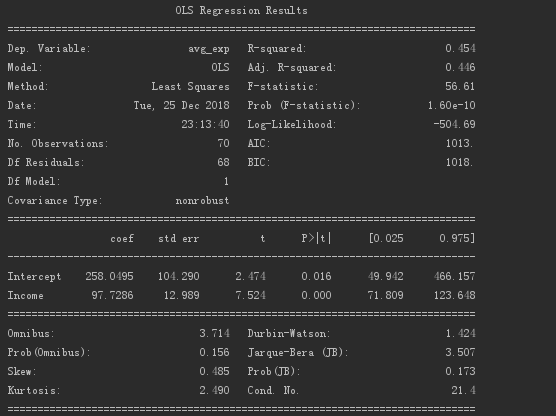
It can be seen from the above that the regression coefficient value is 97.73, and the intercept value is 258.05.
The model outline is as follows.

The R² value is 0.454, and the P value is close to 0, so the model still has a certain reference significance.
Use the linear regression model to test the training data set and get its predicted value and residual error.
# The generated model uses predict to generate predicted values,resid is the residual of the training data set
print(pd.DataFrame([lm_s.predict(exp), lm_s.resid], index=['predict','resid']).T.head())
The output result can be compared with the output result when the data was first read.

Use model testing to predict the outcome of the data set.
# Use the model to predict the data set to be predicted
print(lm_s.predict(exp_new)[:5])
Output the result.

02 Multiple linear regression
Multiple linear regression is based on simple linear regression, adding more independent variables.
Binary linear regression is the simplest multiple linear regression.
One variable regression fits a regression line, then the binary regression fits a regression plane.
In multiple linear regression, a linear relationship between the independent variable and the dependent variable is required, and the correlation coefficient between the independent variables should be as low as possible.
The more independent variables linearly related to the dependent variable in the regression equation, the stronger the interpretation of the regression.
If there are more non-linearly related independent variables in the equation, the weaker the model interpretation is.
The adjusted R² (related to the number of observations and the number of independent variables of the model) can be used to evaluate the pros and cons of the regression, that is, to evaluate the explanatory strength of the model**.
The following is the case in the book to achieve a multiple linear regression.
Analyze the relationship between customer age, annual income, community house average price, local per capita income and credit card monthly average expenditure.
# Use multiple linear regression to build a model
lm_m =ols('avg_exp ~ Age + Income + dist_home_val + dist_avg_income', data=exp).fit()print(lm_m.summary())
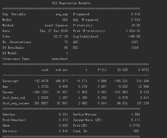
The multiple linear regression model information is as follows.

Output R² is 0.542, adjust R² to 0.513.
The test P value of the equation's significance (the regression coefficient is not all 0) is 1.82e-10, which is close to 0, indicating that the regression equation is meaningful.
The regression coefficients of customer age and average housing price are not significant.
The regression coefficients of annual income and local income per capita are significant.
Multiple linear regression can filter independent variables according to forward method, backward method, and stepwise method.
The forward method is to continuously add variables to construct the regression equation, and the backward rule is to continuously remove the variables to construct the regression equation. The stepwise method is a combination of the two, adding and deleting.
The three methods are based on the AIC criterion (minimum information criterion), where the smaller the AIC value, the better the model effect and the more concise.
Using the AIC criterion can prevent the increase of variables from becoming the main reason for the reduction of the residual sum of squares, and prevent the increase of model complexity.
This time, the forward regression method is used to continuously add variables to obtain the AIC value of the added variables, and finally find the variable with the most explanatory power.
# Forward regression
def forward_select(data, response):"""data is data containing independent variables and dependent variables,response is the dependent variable"""
 # Get list of arguments
 remaining =set(data.columns)
 remaining.remove(response)
 selected =[]
 # Define data type(Positive infinity)
 current_score, best_new_score =float('inf'),float('inf')
 # When the argument list contains arguments
 while remaining:
  aic_with_candidates =[]
  # Loop through the list of arguments
  for candidates in remaining:
   # Build expression,The independent variable will continue to increase
   formula ="{} ~ {}".format(response,' + '.join(selected +[candidates]))
   # AIC interpretation strength of the independent variable generated
   aic =ols(formula=formula, data=data).fit().aic
   # Get the AIC explanation strength list of the independent variable
   aic_with_candidates.append((aic, candidates))
  # Sort the interpretation strength list from largest to smallest
  aic_with_candidates.sort(reverse=True)
  # Get the maximum explained strength(Minimum AIC value)And independent variables
  best_new_score, best_candidate = aic_with_candidates.pop()
  # 1. Positive infinity is greater than the maximum explanatory power 2.The AIC value of the previous experiment must be greater than that of the next experiment,That is, the more variables you add,The AIC value should be smaller,The better the model
  if current_score > best_new_score:
   # Remove the most influential independent variables
   remaining.remove(best_candidate)
   # Add influential independent variables
   selected.append(best_candidate)
   # Assign the AIC value of this experiment
   current_score = best_new_score
   print('aic is {},continue!'.format(current_score))else:print('forward selection over!')break
 # Use a list of influential independent variables,Perform linear regression on the data
 formula ="{} ~ {}".format(response,' + '.join(selected))print('final formula is {}'.format(formula))
 model =ols(formula=formula, data=data).fit()return model

# Use forward regression to filter variables,Use the selected variables to build a regression model
data_for_select = exp[['avg_exp','Income','Age','dist_home_val','dist_avg_income']]
lm_m =forward_select(data=data_for_select, response='avg_exp')print(lm_m.rsquared)
Output the result.

It is found that customer age (Age) is eliminated, and a linear regression model is finally obtained.
/ 03 / Summary
Here is just building a linear regression model, it can only be said to be useful.
The model will be diagnosed later to make the model more valuable.
To be continued...
Recommended Posts