Python Data Science: Neural Networks

( Artificial Neural Network (ANN) artificial neural network model, which simplifies, abstracts and simulates the human brain neural network with mathematical and physical methods.

This time is just a simple introduction to neural networks, involving neuron models and BP neural networks.

Here is a brief look at the three elements of machine learning, namely model, strategy and algorithm.

The model includes the non-random effect part (the relationship between the explained variable and the explanatory variable, mostly a functional relationship) and the random effect part (disturbance term).

Strategy refers to how to set the optimal objective function. Common objective functions include the residual sum of squares of linear regression, the likelihood function of logistic regression, and the hinge function in SVM.

Algorithm is a method of finding parameters for the objective function, such as calculating by derivation, or using algorithms in the field of numerical calculation.

Among them, the neural network uses numerical algorithms to solve the parameters, which means that the model parameters obtained by each calculation will be different.

/ 01 / Neural Network

01 Neuron model

The most basic component in a neural network is the neuron model.

Each neuron is a multiple input single output information processing unit. The input signal is transmitted through a weighted connection, and the total input value is obtained after comparison with the threshold, and then a *single output is generated through the activation function processing *.

The output of the neuron is the result of applying a weighted sum of inputs to the activation function.

The activation function of the neuron makes the neuron have different information processing characteristics, reflecting the relationship between the output of the neuron and its activation state.

The activation functions involved this time include threshold function (step function) and sigmoid function (sigmoid function).

02 Single layer perceptron

The perceptron is a neural network with a single-layer computing unit, which can only be used to solve linearly separable binary classification problems.

It cannot be applied to a multilayer perceptron, and the expected output of the hidden layer cannot be determined.

Its structure is similar to the previous neuron model.

The activation function uses a unipolar (or bipolar) threshold function.

03 BP neural network

The multi-layer neural network trained with error back propagation algorithm (supervised learning algorithm) is called BP neural network.

It belongs to a multi-layer feedforward neural network. The learning process of the model consists of two processes of signal forward propagation and error back propagation.

When the signal is propagated forward, the weighted sum of each layer is calculated from the input layer, and finally transferred to the output layer through each hidden layer to obtain the output result. The output result is compared with the expected result (supervision signal) to obtain the output error.

Error backpropagation is based on the gradient descent algorithm to propagate the error back layer by layer along the hidden layer to the input layer, apportion the error to all units of each layer, so as to obtain the error signal (learning signal) of each unit, and modify each unit accordingly. Unit weight.

These two signal propagation processes continuously loop to update the weight, and finally determine whether to end the loop according to the judgment condition.

The network structure is generally a single hidden layer network, including input layer, hidden layer, and output layer.

The activation function mostly uses a sigmoid function or a linear function, where both the hidden layer and the output layer use the sigmoid function.

/ 02/ Python implementation

After the neural network has clear training samples, the input layer node number (the number of explanatory variables) and the output layer node number (the number of explained variables) of the network have been determined.

What needs to be considered is the number of hidden layers and the number of nodes in each hidden layer.

Let's use the data in the book to carry out a wave of actual combat, a mobile off-grid data.

Mobile communication user consumption characteristics data, the target field is whether to churn, with two classification levels (yes or not).

The independent variables include the user's basic information, the product information consumed, and the user's consumption characteristics.

Read the data.

import pandas as pd
from sklearn import metrics
import matplotlib.pyplot as plt
from sklearn.preprocessing import MinMaxScaler
from sklearn.neural_network import MLPClassifier
from sklearn.model_selection import GridSearchCV
from sklearn.model_selection import train_test_split

# Set the maximum number of displayed lines
pd.set_option('display.max_rows',10)
# Set the maximum number of displayed columns
pd.set_option('display.max_columns',10)
# Set the display width to 1000,This way it won't wrap in the IDE
pd.set_option('display.width',1000)
# Read data,skipinitialspace:Ignore white space after delimiter
churn = pd.read_csv('telecom_churn.csv', skipinitialspace=True)print(churn)

Output data overview, including more than 3000 user data.

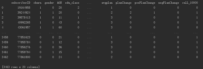
Use the functions in scikit-learn to divide the data set into a training set and a test set.

# Select independent variable data
data = churn.iloc[:,2:]
# Select dependent variable data
target = churn['churn']
# Use scikit-learn divides the data set into a training set and a test set
train_data, test_data, train_target, test_target =train_test_split(data, target, test_size=0.4, train_size=0.6, random_state=1234)

The neural network needs to extreme normalization of the data.

Continuous variables need to be standardized with extreme values, and categorical variables need to be transformed into dummy variables.

Among them, multi-category nominal variables must be converted into dummy variables, while grade variables and binary categorical variables can choose not to change, and can be treated as continuous variables.

In this data, education level and package type are grade variables, and variables such as gender are binary variables, which can be treated as continuous variables.

This also means that there are no multi-categorical nominal variables in this data set, and they can all be treated as continuous variables.

# Extreme value normalization
scaler =MinMaxScaler()
scaler.fit(train_data)

scaled_train_data = scaler.transform(train_data)
scaler_test_data = scaler.transform(test_data)

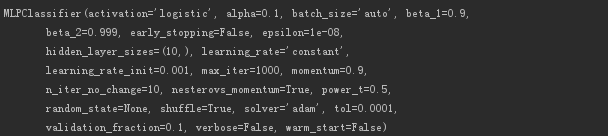
Build a multilayer perceptron model.

# Set the model corresponding to the multilayer perceptron
mlp =MLPClassifier(hidden_layer_sizes=(10,), activation='logistic', alpha=0.1, max_iter=1000)
# Model training on the training set
mlp.fit(scaled_train_data, train_target)
# Output neural network model information
print(mlp)

The output model information is as follows.

Next, use the model trained on the training set to make predictions on the training set and test set.

# Use the model to make predictions
train_predict = mlp.predict(scaled_train_data)
test_predict = mlp.predict(scaler_test_data)

Output predicted probability, the probability of user loss.

# Output model prediction probability(1 case)
train_proba = mlp.predict_proba(scaled_train_data)[:,1]
test_proba = mlp.predict_proba(scaler_test_data)[:,1]

Evaluate the model and output the evaluation data.

# Output model evaluation results based on prediction information
print(metrics.confusion_matrix(test_target, test_predict, labels=[0,1]))print(metrics.classification_report(test_target, test_predict))

The output is as follows.

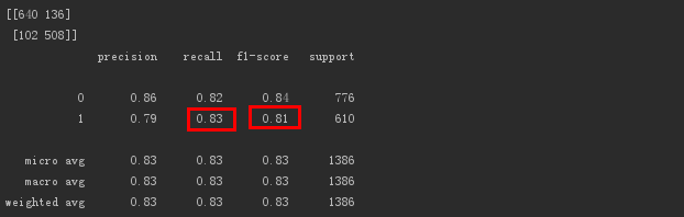
The model's f1-score (harmonized average of precision rate and recall rate) value for lost users is 0.81, and the effect is good.

In addition, the sensitivity recall for lost users is 0.83, and the model can identify 83% of lost users, indicating that the model's ability to identify lost users is acceptable.

The average accuracy of the output model prediction.

# Use the specified data set to output the average accuracy of the model prediction
print(mlp.score(scaler_test_data, test_target))
# Output value is 0.8282828282828283

The average accuracy value is 0.8282.

Calculate the area under the ROC of the model.

# Draw ROC curve
fpr_test, tpr_test, th_test = metrics.roc_curve(test_target, test_proba)
fpr_train, tpr_train, th_train = metrics.roc_curve(train_target, train_proba)
plt.figure(figsize=[3,3])
plt.plot(fpr_test, tpr_test,'b--')
plt.plot(fpr_train, tpr_train,'r-')
plt.title('ROC curve')
plt.show()

# Calculate AUC value
print(metrics.roc_auc_score(test_target, test_proba))
# Output value is 0.9149632415075206

The ROC curve is as follows.

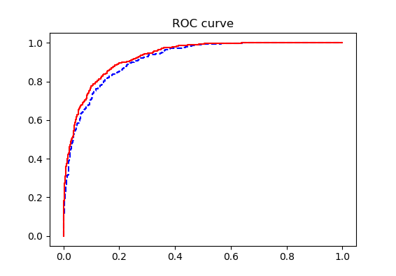
The curves of the training set and the test set are very close, and there is no over-fitting phenomenon.

The AUC value is 0.9149, indicating that the model is very effective.

Search for the optimal parameters of the model, and train the model under the optimal parameters.

# Use GridSearchCV for optimal parameter search
param_grid ={
 # Number of hidden layers in the model
 ' hidden_layer_sizes':[(10,),(15,),(20,),(5,5)],
 # Activation function
 ' activation':['logistic','tanh','relu'],
 # Regularization coefficient
 ' alpha':[0.001,0.01,0.1,0.2,0.4,1,10]}

mlp =MLPClassifier(max_iter=1000)
# Choose roc_auc as the criterion,4-fold cross validation,n_jobs=-1 Use all threads of a multi-core CPU
gcv =GridSearchCV(estimator=mlp, param_grid=param_grid,
     scoring='roc_auc', cv=4, n_jobs=-1)
gcv.fit(scaled_train_data, train_target)

The case of the model that outputs the optimal parameters.

# Output the score of the model under the optimal parameters
print(gcv.best_score_)
# Output value is 0.9258018987136855

# Output the parameters of the model under the optimal parameters
print(gcv.best_params_)
# The output parameter value is{'alpha':0.01,'activation':'tanh','hidden_layer_sizes':(5,5)}

# Use the specified data set to output the average accuracy of the optimal model prediction
print(gcv.score(scaler_test_data, test_target))
# Output value is 0.9169384823390232

The model's highest score of roc_auc is 0.92, that is, the area under the ROC curve under this model is 0.92.

Compared with the previous 0.9149, it has improved a little.

The optimal parameters of the model, the activation function is relu type, the alpha is 0.01, and the number of hidden layer nodes is 15.

The average prediction accuracy of the model is 0.9169, which is much higher than the previous 0.8282.