Python Data Science: Regularization Methods

Following the previous linear regression article, the portal is as follows.

[ Python Data Science: Linear Regression Diagnosis](http://mp.weixin.qq.com/s?__biz=MzU4OTYzNjE2OQ==&mid=2247484309&idx=1&sn=156ca4967d967a164abeab7009faab20&chksm=fdcb34b3cabcbda503c751c80db6bae1615

The above article uses the variance inflation factor to diagnose and reduce the impact of multicollinearity on linear regression.

Human intervention is required (judging according to the obtained variance inflation value), which consumes too much time.

So there is the emergence of the regularization method, and regression is carried out through the shrinkage method (regularization method).

Regularization methods mainly include ridge regression and LASSO regression.

/ 01 / Ridge Return

Ridge regression estimates the regression coefficients through ** artificially added penalty terms (constraints) **, which is a biased estimate.

Biased estimation allows the estimation to have a small degree of skewness in exchange for a significant reduction in the estimated error, and the regression coefficient is estimated under the principle of the minimum sum of squared residuals.

Usually R² in the ridge regression equation will be slightly lower than linear regression analysis, but the significance of the regression coefficient is often significantly higher than that of ordinary linear regression.

The corresponding theoretical knowledge is not elaborated here. To be honest, Little F is also dizzy...

So choose to adjust the package first to see what the effect is.

The machine learning framework scikit-learn is used to select ridge regression parameters (regularization coefficients).

The data is the data in the book. It has been uploaded to the web disk, and the official account will reply "Regularization" to obtain it.

The model in scikit-learn does not standardize the data by default and must be executed manually.

The standardized data can eliminate the dimension, allowing the coefficient of each variable to be directly compared in a certain sense.

import numpy as np
import pandas as pd
import matplotlib.pyplot as plt
from sklearn.linear_model import Ridge
from sklearn.linear_model import RidgeCV
from sklearn.preprocessing import StandardScaler

# Eliminate pandas output ellipsis and line breaks
pd.set_option('display.max_columns',500)
pd.set_option('display.width',1000)
# Read data,skipinitialspace:Ignore white space after delimiter
df = pd.read_csv('creditcard_exp.csv', skipinitialspace=True)
# Get line data of credit card expenditure
exp = df[df['avg_exp'].notnull()].copy().iloc[:,2:].drop('age2', axis=1)
# Get row data of credit card without expenditure,NaN
exp_new = df[df['avg_exp'].isnull()].copy().iloc[:,2:].drop('age2', axis=1)

# Choose 4 continuous variables,Respectively, age income, local community price, local per capita income
continuous_xcols =['Age','Income','dist_home_val','dist_avg_income']
# standardization
scaler =StandardScaler()
# Explanatory variables,Two-dimensional array
X = scaler.fit_transform(exp[continuous_xcols])
# Explained variable,One-dimensional array
y = exp['avg_exp_ln']

# Generate regularization coefficient
alphas = np.logspace(-2,3,100, base=10)
# Cross-validate the model with different regularization coefficients
rcv =RidgeCV(alphas=alphas, store_cv_values=True)
# Use data set training(fit)
rcv.fit(X, y)
# Output optimal parameters,Regularization coefficient and corresponding model R²
print('The best alpha is {}'.format(rcv.alpha_))print('The r-square is {}'.format(rcv.score(X, y)))

# After training, use transform for data conversion
X_new = scaler.transform(exp_new[continuous_xcols])
# Use models to make predictions on data
print(np.exp(rcv.predict(X_new)[:5]))

The output is as follows.

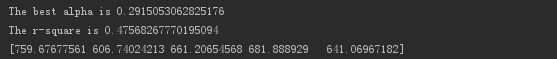
The optimal regularization coefficient is 0.29, and the model R² is 0.475.

And use the ridge regression model under the optimal regularization coefficient to predict the data.

Visualize the mean square error of the model under different regularization coefficients.

# The result of each round of cross validation in the regularization coefficient search space,Mean square error of the model
cv_values = rcv.cv_values_
n_fold, n_alphas = cv_values.shape
# Model mean square error fluctuation value
cv_mean = cv_values.mean(axis=0)
cv_std = cv_values.std(axis=0)
ub = cv_mean + cv_std / np.sqrt(n_fold)
lb = cv_mean - cv_std / np.sqrt(n_fold)
# Draw a line chart,The x-axis is in exponential form
plt.semilogx(alphas, cv_mean, label='mean_score')
# y1(lb)And y2(ub)Fill in between
plt.fill_between(alphas, lb, ub, alpha=0.2)
plt.xlabel('$\\alpha$')
plt.ylabel('mean squared errors')
plt.legend(loc='best')
plt.show()

The output is as follows.

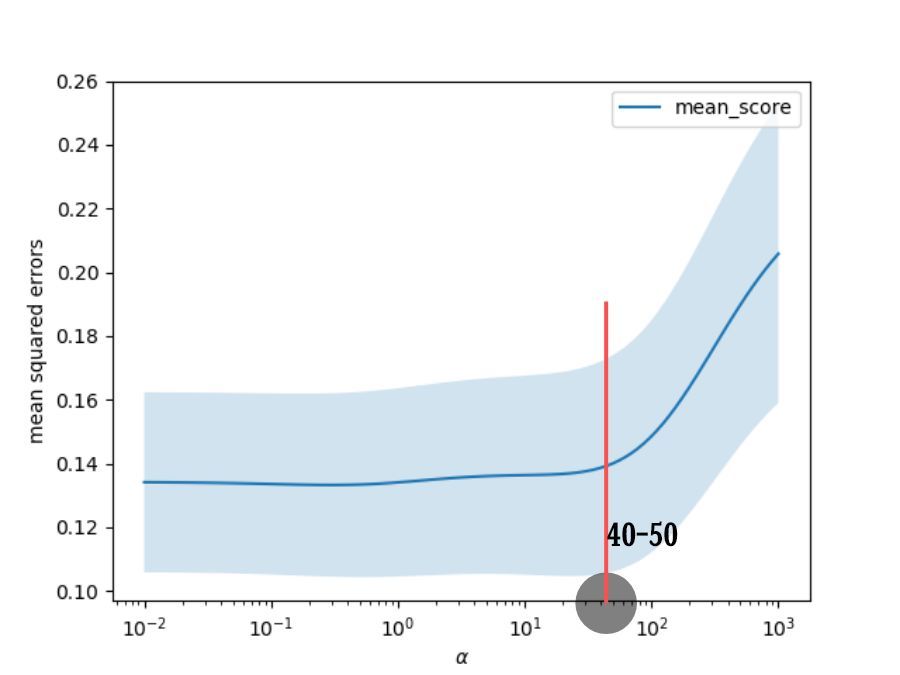
It is found that when the regularization coefficient is below 40 or 50, the mean square error of the model is not much different.

When the coefficient exceeds the threshold, the mean square error increases rapidly.

So as long as the regularization coefficient is less than 40 or 50, the fitting effect of the model should be good.

**The smaller the regularization coefficient, the better the model fit, but the more likely to happen over-fitting. **

**The larger the regularization coefficient, the less likely it is to overfit, but the greater the deviation of the model. **

RidgeCV can quickly return to the "optimal" regularization coefficient through cross-validation.

When this is only based on numerical calculations, the final result may not conform to business logic.

For example, the variable coefficients of this model.

# Variable coefficient of output model
print(rcv.coef_)
# Output result
[0.03321449-0.309561850.055512080.59067449]

It is definitely unreasonable to find that the coefficient of income is negative.

The following is a further analysis through the ridge trace diagram.

The ridge trace diagram is the trajectory of variable coefficients under different regularization coefficients.

ridge =Ridge()
coefs =[]
# Variable coefficients under different regularization coefficients
for alpha in alphas:
 ridge.set_params(alpha=alpha)
 ridge.fit(X, y)
 coefs.append(ridge.coef_)

# Plot the trajectory of the variable coefficient with the regularization coefficient
ax = plt.gca()
ax.plot(alphas, coefs)
ax.set_xscale('log')
plt.xlabel('alpha')
plt.ylabel('weights')
plt.title('Ridge coefficients as a function of the regularization')
plt.axis('tight')
plt.show()

Output the result.

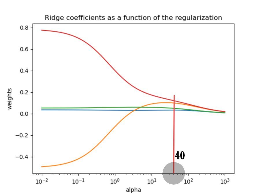
①The coefficients of two variables are very close to 0 under different regularization coefficients, so you can choose to delete them.

②The greater the regularization coefficient, the greater the penalty for the variable coefficient, and the coefficients of all variables tend to be zero.

③The coefficient of a variable has a very large change (positive and negative), indicating that the variance of the coefficient is large and there is collinearity.

Integrating the mean square error of the model and the ridge trace map, the regularization coefficient is selected as 40.

**If it is greater than 40, the mean square error of the model increases and the model fitting effect becomes worse. **

**If it is less than 40, the variable coefficient is unstable and collinearity is not suppressed. **

Then let's take a look, when the regularization coefficient is 40, the model variable coefficients.

ridge.set_params(alpha=40)
ridge.fit(X, y)
# Output variable coefficient
print(ridge.coef_)
# Output model R²
print(ridge.score(X, y))
# Forecast data
print(np.exp(ridge.predict(X_new)[:5]))
# Output result
[0.032931090.099077470.049763050.12101456]0.4255673043353688[934.79025945727.11042209703.88143602759.04342764709.54172995]

It is found that the variable coefficients are all positive, which is in line with business intuition.

The two variables, income and local income per capita, can be kept, and the other two are deleted.

/ 02/ LASSO returns

LASSO regression minimizes the residual sum of squares under the constraint condition that the sum of the absolute values of the regression coefficients is less than a constant.

Thus, some regression coefficients strictly equal to 0 can be generated, and a model with strong explanatory power can be obtained.

Compared with ridge regression, LASSO regression can also perform variable screening.

Use LassoCV cross-validation to determine the optimal regularization coefficient.

# Generate regularization coefficient
lasso_alphas = np.logspace(-3,0,100, base=10)
# Cross-validate the model with different regularization coefficients
lcv =LassoCV(alphas=lasso_alphas, cv=10)
# Use data set training(fit)
lcv.fit(X, y)
# Output optimal parameters,Regularization coefficient and corresponding model R²
print('The best alpha is {}'.format(lcv.alpha_))print('The r-square is {}'.format(lcv.score(X, y)))

# Output result
The best alpha is 0.04037017258596556
The r-square is 0.4426451069862233

It is found that the optimal regularization coefficient is 0.04, and the model R² is 0.443.

Next, obtain the variable coefficient trajectory under different regularization coefficients.

lasso =Lasso()
lasso_coefs =[]
# Variable coefficients under different regularization coefficients
for alpha in lasso_alphas:
 lasso.set_params(alpha=alpha)
 lasso.fit(X, y)
 lasso_coefs.append(lasso.coef_)

# Plot the trajectory of the variable coefficient with the regularization coefficient
ax = plt.gca()
ax.plot(lasso_alphas, lasso_coefs)
ax.set_xscale('log')
plt.xlabel('alpha')
plt.ylabel('weights')
plt.title('Lasso coefficients as a function of the regularization')
plt.axis('tight')
plt.show()

Output the result.

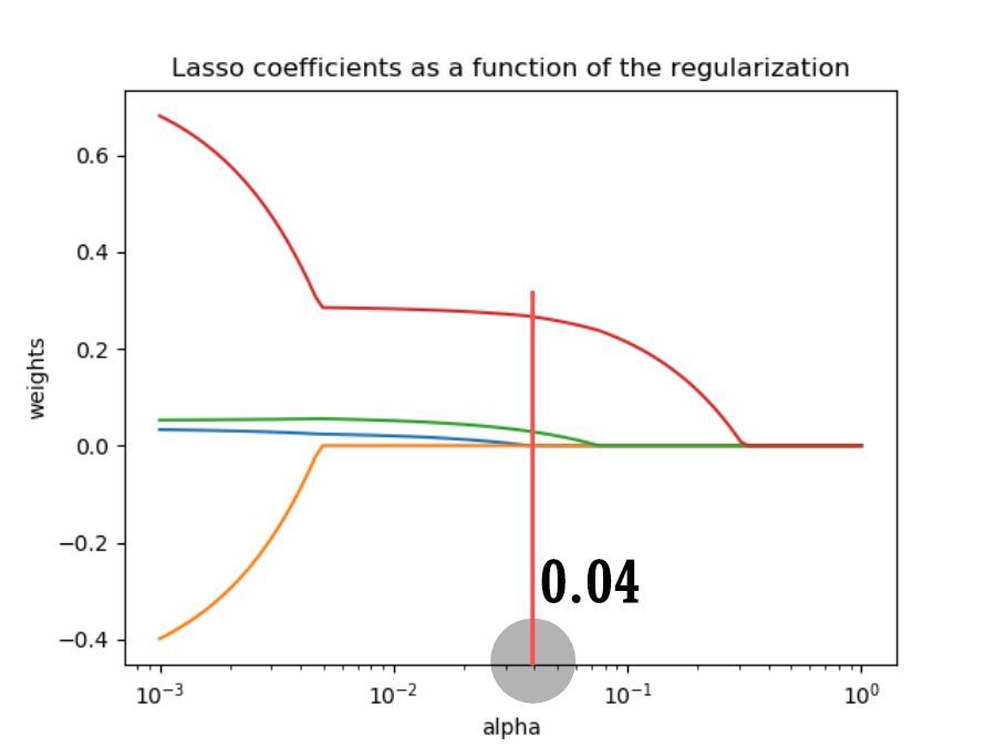
It is found that as the regularization coefficient increases, the coefficients of all variables will suddenly drop to 0 at a certain threshold.

The reason is related to the LASSO regression equation and will not be elaborated.

Output the variable coefficients of LASSO regression.

print(lcv.coef_)
# Output result
[0.0.0.027894890.26549855]

It is found that the first two variables have been filtered out, namely age and income.

Why is the result different from Ling Regression? ? ?