Python analysis of wav files
For the analysis of sound files, in addition to listening, it is best to convert the sound into graphics, so that there is a visual perception of the difference between the sound files, which can be a very useful supplement for subsequent analysis.
Python can use SCIPY library to load wav files and use matplotlib to draw graphics. First I downloaded 1M and 2M wav files from this website as wav sample files: https://file-examples.com/index.php/sample-audio-files/sample-wav-download/
Then use the following code to install and draw the tonal graph of the wav file:
from scipy.io import wavfile
from matplotlib import pyplot as plt
from matplotlib.pyplot import figure

# load wav files
fs_1m,data_1m = wavfile.read("./wav/file_example_WAV_1MG.wav")
fs_2m,data_2m = wavfile.read("./wav/file_example_WAV_2MG.wav")

# set plt style
plt.style.use('seaborn-whitegrid')

# plot data
fig,(ax1, ax2)= plt.subplots(1,2)
ax1.plot(data_1m, color='b')
ax1.set_title("auido with 1M size")
ax2.plot(data_2m, color='y')
ax2.set_title("auido with 2M size")

plt.savefig('audio.png', dpi=150)
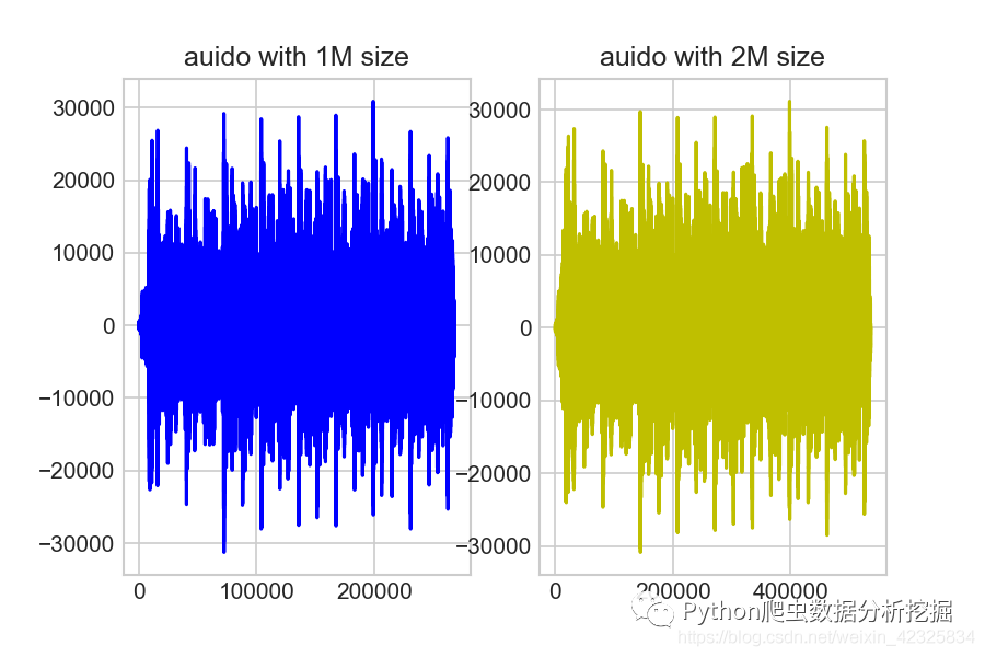
The output graphics are as follows:

It can be seen that the two graphics are basically the same, but the X coordinate of the 2M file is twice that of the 1M file.
Then we can easily calculate the Euclidean distance between two audio data using the fastdtw library:
from fastdtw import fastdtw
from scipy.spatial.distance import euclidean

# calculate euclidean distance
distance,path =fastdtw(data_1m, data_2m, dist=euclidean)print("the distance between the two clips is %s"% distance)
The output is as follows:
the distance between the two clips is 4093034781.337242
Recommended Posts