Python implements threshold regression
The basic idea of the Threshold Regressive Model (TR model or TRM) is to use the control function of the threshold variable. When the predictor data is given, the threshold value of the threshold variable first determines the control function according to the threshold value of the threshold variable. Use different forecasting equations to try to explain various phenomena like jumps and sudden changes. Its essence is to classify the forecasting problems according to the value of the state space, and use the piecewise linear regression model to describe the overall nonlinear forecasting problem.
The modeling step of multiple threshold regression is the process of confirming the threshold variables, calibrating the threshold number L, the threshold value and the regression coefficient. For the convenience of calculation, two divisions (ie L=2) are used to illustrate the modeling steps of the model.
The basic steps are as follows (with code):
- Read the data and calculate the correlation coefficient matrix between the forecast object and the forecast factor.
Data read
# Use pandas to read csv, the data read is a DataFrame object
data = pd.read_csv('jl.csv')
# Convert DataFrame object to array,The first column of the array is the data number, the last column is the forecast object, and the middle columns are the forecast factors
data= data.values.copy()
# print(data)
# Calculate the cross-correlation coefficient, the parameters are the predictor sequence and the lag time k
def get_regre_coef(X,Y,k):
 S_xy=0
 S_xx=0
 S_yy=0
 # Calculate the mean value of forecast factors and forecast objects
 X_mean = np.mean(X)
 Y_mean = np.mean(Y)for i inrange(len(X)-k):
 S_xy +=(X[i]- X_mean)*(Y[i+k]- Y_mean)for i inrange(len(X)):
 S_xx +=pow(X[i]- X_mean,2)
 S_yy +=pow(Y[i]- Y_mean,2)return S_xy/pow(S_xx*S_yy,0.5)
# Calculate the correlation coefficient matrix
def regre_coef_matrix(data):
 row=data.shape[1]#Number of columns
 r_matrix=np.ones((1,row-2))
 # print(row)for i inrange(1,row-1):
 r_matrix[0,i-1]=get_regre_coef(data[:,i],data[:,row-1],1)#Lag time is 1 return r_matrix
r_matrix=regre_coef_matrix(data)
# print(r_matrix)
### Output###
#[[0.0489790.078299890.190057050.275012090.28604638]]
- The correlation coefficients are sorted, and the factor with the largest correlation coefficient is used as the threshold element.
# Sort the correlation coefficient and find the largest correlation coefficient as the threshold element
def get_menxiannum(r_matrix):
 row=r_matrix.shape[1]#Number of columns
 for i inrange(row):if r_matrix.max()==r_matrix[0,i]:return i+1return-1
m=get_menxiannum(r_matrix)
# print(m)
## Output##The fifth factor has the largest correlation coefficient
#5
- Reorder the data according to the selected threshold element factor.
# Sort the factor sequence according to the threshold element,m is the serial number of the threshold variable
def resort_bymenxian(data,m):
 data=data.tolist()#Convert to list
 data.sort(key=lambda x: x[m])#List according to m+1 column to sort(Ascending)
 data=np.array(data)return data
data=resort_bymenxian(data,m)#Get the sorted sequence array
- The sorted sequence is divided into two segments according to the threshold element, the first segment is 1 data, the second segment is n-1 (n is the sample capacity) data; the second segment is 2 data, The second segment of n-2 data, one-time analogy, respectively calculate the divided F statistic and select the segmentation point of the threshold element corresponding to the largest statistic as the threshold.
def get_var(x):return x.std()**2* x.size #Calculate the total variance
# Calculation of statistic F,The input data is the forecast object data sorted according to the threshold element
def get_F(Y):
 col=Y.shape[0]#Number of rows, sample size
 FF=np.ones((1,col-1))#Store statistics of different split points
 V=get_var(Y)#Calculate the total variance
 for i inrange(1,col):#1 to col-1
 S=get_var(Y[0:i])+get_var(Y[i:col])#Calculate the sum of variance within two segments
 F=(V-S)*(col-2)/S
 FF[0,i-1]=F#At this step, it is necessary to judge whether the F test is passed, and the F statistic is retained only after passing
 return FF
y=data[:,data.shape[1]-1]
FF=get_F(y)
def get_index(FF,element):#Get the index of the first occurrence of element in a one-dimensional array FF
 i=-1for item in FF.flat:
 i+=1if item==element:return i
f_index=get_index(FF,np.max(FF))#Get the largest index of the statistic F
# print(data[f_index,m-1])#The threshold element is the fifth factor, and the threshold value is 121 when substituted into the index
- The data sequence is divided into two segments with the threshold as the dividing point, and multiple linear regression is performed respectively. Here, the linear regression module in the sklearn.linear_model module is used. Substituting the predictive factors to calculate the predicted values of the two segments respectively.
# Divide the new data sequence into two parts with the threshold as the dividing point, and perform multiple regression calculations respectively
def data_excision(data,f_index):
 f_index=f_index+1
 data1=data[0:f_index,:]
 data2=data[f_index:data.shape[0],:]return data1,data2
data1,data2=data_excision(data,f_index)
# First paragraph
def get_XY(data):
 # Array slice to assign values to variables
 Y = data[:, data.shape[1]-1] #The forecast object is in the last column
 X = data[:,1:data.shape[1]-1]#Predictor from the second column to the penultimate column
 return X, Y
X,Y=get_XY(data1)
regs=LinearRegression()
regs.fit(X,Y)
# print('First paragraph')
# print(regs.coef_)#Output regression coefficient
# print(regs.score(X,Y))#Output correlation coefficient
# Calculate predicted value
Y1=regs.predict(X)
# print('Second paragraph')
X,Y=get_XY(data2)
regs.fit(X,Y)
# print(regs.coef_)#Output regression coefficient
# print(regs.score(X,Y))#Output correlation coefficient
# Calculate predicted value
Y2=regs.predict(X)
Y=np.column_stack((data[:,0],np.hstack((Y1,Y2)))).copy()
Y=np.column_stack((Y,data[:,data.shape[1]-1]))
Y=resort_bymenxian(Y,0)
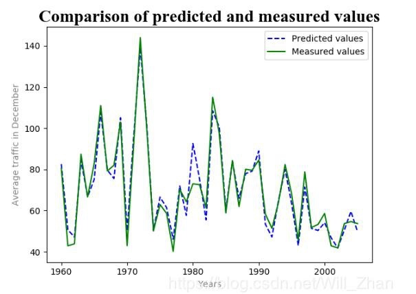
- The predicted value and the actual value are re-sorted according to the year number, the order is restored, and the matplotlib module is used to make a comparison chart between the predicted value and the actual value.
# Recovery order
Y=resort_bymenxian(Y,0)
# print(Y.shape)
# Visualization of forecast results
plt.plot(Y[:,0],Y[:,1],'b--',Y[:,0],Y[:,2],'g')
plt.title('Comparison of predicted and measured values',fontsize=20,fontname='Times New Roman')#Add title
plt.xlabel('Years',color='gray')#Add x-axis label
plt.ylabel('Average traffic in December',color='gray')#Add y-axis label
plt.legend(['Predicted values','Measured values'])#Add legend
plt.show()
Result graph:
Data used: Quoted from "Modern Medium and Long-term Hydrological Forecasting Methods and Applications" by Zhang Shiming, Tang Chengyou's official article
| num | x1 | x2 | x3 | x4 | x5 | y |
|---|---|---|---|---|---|---|
| 1960 | 308 | 301 | 352 | 310 | 149 | 80.5 |
| 1961 | 182 | 186 | 165 | 127 | 70 | 42.9 |
| 1962 | 195 | 134 | 134 | 97 | 61 | 43.9 |
| 1963 | 136 | 378 | 334 | 307 | 148 | 87.4 |
| 1964 | 230 | 630 | 332 | 161 | 100 | 66.6 |
| 1965 | 225 | 333 | 209 | 365 | 152 | 82.9 |
| 1966 | 296 | 225 | 317 | 527 | 228 | 111 |
| 1967 | 324 | 229 | 176 | 317 | 153 | 79.3 |
| 1968 | 278 | 230 | 352 | 317 | 143 | 82 |
| 1969 | 662 | 442 | 453 | 381 | 188 | 103 |
| 1970 | 187 | 136 | 103 | 129 | 74.7 | 43 |
| 1971 | 284 | 404 | 600 | 327 | 161 | 92.2 |
| 1972 | 427 | 430 | 843 | 448 | 236 | 144 |
| 1973 | 258 | 404 | 639 | 275 | 156 | 98.9 |
| 1974 | 113 | 160 | 128 | 177 | 77.2 | 50.1 |
| 1975 | 143 | 300 | 333 | 214 | 106 | 63 |
| 1976 | 113 | 74 | 193 | 241 | 107 | 58.6 |
| 1977 | 204 | 140 | 154 | 90 | 55.1 | 40.2 |
| 1978 | 174 | 445 | 351 | 267 | 120 | 70.3 |
| 1979 | 93 | 95 | 197 | 214 | 94.9 | 64.3 |
| 1980 | 214 | 250 | 354 | 385 | 178 | 73 |
| 1981 | 232 | 676 | 483 | 218 | 113 | 72.6 |
| 1982 | 266 | 216 | 146 | 112 | 82.8 | 61.4 |
| 1983 | 210 | 433 | 803 | 301 | 166 | 115 |
| 1984 | 261 | 702 | 512 | 291 | 153 | 97.5 |
| 1985 | 197 | 178 | 238 | 180 | 94.2 | 58.9 |
| 1986 | 442 | 256 | 623 | 310 | 146 | 84.3 |
| 1987 | 136 | 99 | 253 | 232 | 114 | 62 |
| 1988 | 256 | 226 | 185 | 321 | 151 | 80.1 |
| 1989 | 473 | 409 | 300 | 298 | 141 | 79.6 |
| 1990 | 277 | 291 | 639 | 302 | 149 | 84.6 |
| 1991 | 372 | 181 | 174 | 104 | 68.8 | 58.4 |
| 1992 | 251 | 142 | 126 | 95 | 59.4 | 51.4 |
| 1993 | 181 | 125 | 130 | 240 | 121 | 64 |
| 1994 | 253 | 278 | 216 | 182 | 124 | 82.4 |
| 1995 | 168 | 214 | 265 | 175 | 101 | 68.1 |
| 1996 | 98.8 | 97 | 92.7 | 88 | 56.7 | 45.6 |
| 1997 | 252 | 385 | 313 | 270 | 119 | 78.8 |
| 1998 | 242 | 198 | 137 | 114 | 71.9 | 51.8 |
| 1999 | 268 | 178 | 127 | 109 | 68.6 | 53.3 |
| 2000 | 86.2 | 286 | 233 | 133 | 77.8 | 58.6 |
| 2001 | 150 | 168 | 122 | 93 | 62.8 | 42.9 |
| 2002 | 180 | 150 | 97.8 | 78 | 48.2 | 41.9 |
| 2003 | 166 | 203 | 166 | 124 | 70 | 53.7 |
| 2004 | 400 | 202 | 126 | 158 | 92.7 | 54.7 |
| 2005 | 79.8 | 82.6 | 129 | 160 | 76.6 | 53.7 |
The above python threshold regression method is all the content shared by the editor, I hope to give you a reference.
Recommended Posts