How to query Prometheus on Ubuntu 14.04 part 1
Introduction
Prometheus is an open source monitoring system and time series database. One of the most important aspects of Prometheus is its multidimensional data model and accompanying query language. This query language allows you to slice and dice dimensional data to answer operational questions in a temporary way, display trends in dashboards, or generate alerts about system failures.
In this tutorial, we will learn how to query Prometheus 1.3.1. In order to use suitable sample data, we will set up three identical demonstration service instances for deriving various synthetic metrics. Then, we will set up a Prometheus server to crawl and store these metrics. Using example metrics, we will learn how to query Prometheus, starting with simple queries and then moving to more advanced queries.
After this tutorial, you will learn how to select and filter time series based on dimensions, aggregate and transform time series, and how to perform arithmetic operations between different indicators. In subsequent tutorials, we will introduce more advanced query use cases based on the knowledge in this tutorial.
Preparation
To follow this tutorial, you need:
- An Ubuntu 14.04 server, including a non-root user with sudo privileges. Students who don’t have a server can buy it from here, but I personally recommend you to use the free Tencent Cloud Developer Lab for experimentation, and then buy server.
Step 1-Install Prometheus
In this step, we will download, configure and run the Prometheus server to scrape three (not yet running) demo service instances.
First, download Prometheus:
wget https://github.com/prometheus/prometheus/releases/download/v1.3.1/prometheus-1.3.1.linux-amd64.tar.gz
Extract the tarball:
tar xvfz prometheus-1.3.1.linux-amd64.tar.gz
Create a minimal Prometheus configuration file on the host file system on ~/prometheus.yml:
nano ~/prometheus.yml
Add the following to the file:
# Scrape the three demo service instances every 5 seconds.
global:
scrape_interval: 5s
scrape_configs:- job_name:'demo'
static_configs:- targets:-'localhost:8080'-'localhost:8081'-'localhost:8082'
Save and exit nano.
This sample configuration caused Prometheus to scrape the demo instance. Prometheus uses a pull model, which is why it needs to be configured to understand the endpoint from which metrics are extracted. The demo instance is not yet running, but it will run on ports 8080, 8081, and 8082 later.
Use nohup and start Prometheus as a background process:
nohup ./prometheus-1.3.1.linux-amd64/prometheus -storage.local.memory-chunks=10000&
Send the output of nohup at the beginning of the command to the file ~/nohup.out instead of stdout. At the end of the command, & will make the process continue to run in the background, while giving you other command prompts. To return the process to the foreground (that is, to the running process of the terminal), use the fg command on the same terminal.
If all goes well, in the ~/nohup.out file, you should see output similar to the following:
time="2016-11-23T03:10:33Z" level=info msg="Starting prometheus (version=1.3.1, branch=master, revision=be476954e80349cb7ec3ba6a3247cd712189dfcb)" source="main.go:75"
time="2016-11-23T03:10:33Z" level=info msg="Build context (go=go1.7.3, user=root@37f0aa346b26, date=20161104-20:24:03)" source="main.go:76"
time="2016-11-23T03:10:33Z" level=info msg="Loading configuration file prometheus.yml" source="main.go:247"
time="2016-11-23T03:10:33Z" level=info msg="Loading series map and head chunks..." source="storage.go:354"
time="2016-11-23T03:10:33Z" level=info msg="0 series loaded." source="storage.go:359"
time="2016-11-23T03:10:33Z" level=warning msg="No AlertManagers configured, not dispatching any alerts" source="notifier.go:176"
time="2016-11-23T03:10:33Z" level=info msg="Starting target manager..." source="targetmanager.go:76"
time="2016-11-23T03:10:33Z" level=info msg="Listening on :9090" source="web.go:240"
In another terminal, you can use the tail -f ~/nohup.out command to monitor the contents of this file. When the content is written to the file, it will be displayed to the terminal.
By default, Prometheus will load its configuration from prometheus.yml (the one we just created) and store its measurement data in ./data in the current working directory.
- The storage.local.memory-chunks flag adjusts the memory usage of Prometheus to a very small amount of RAM (only 512MB) of the host system and a small amount of time series stored in this tutorial.
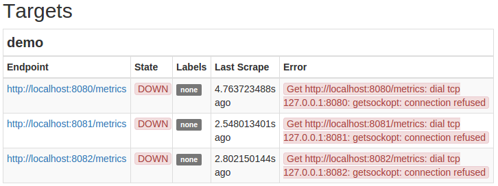
You should now be able to access the Prometheus server at http://your_server_ip:9090/. Verify that it is configured to collect metrics from the three demo instances by pointing to http://your_server_ip:9090/status in the "Target" section and finding the three target endpoints of the demo job. The State column of all three targets should show the status of the target as DOWN, because the demo instance has not been started, so it cannot be deleted:
Step 2-Install the demo example
In this section, we will install and run three demo service instances.
Download demo service:
wget https://github.com/juliusv/prometheus_demo_service/releases/download/0.0.4/prometheus_demo_service-0.0.4.linux-amd64.tar.gz
Extract it:
tar xvfz prometheus_demo_service-0.0.4.linux-amd64.tar.gz
Run the demo service three times on different ports:
. /prometheus_demo_service -listen-address=:8080&./prometheus_demo_service -listen-address=:8081&./prometheus_demo_service -listen-address=:8082&
& will start the demo service in the background. They will not log anything, but they will expose Prometheus metrics on the /metrics HTTP endpoint on their respective ports.
These demonstration services export comprehensive indicators about several simulation subsystems. these are:
- HTTP API server that exposes request count and latency (keyed by path, method and response status code)
- Periodic batch processing job, revealing the timestamp of the last successful run and the number of bytes processed
- Comprehensive indicators on the number of CPUs and their usage
- Comprehensive indicators about the total disk size and its usage
Each indicator is introduced in the query example in the following section.
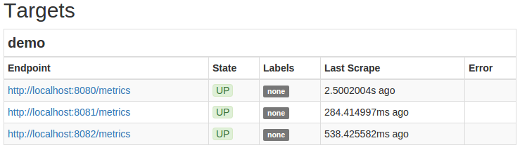
The Prometheus server should now automatically start crawling your three demo instances. Go to the status page of the Prometheus server http://your_server_ip:9090/status``demo, and verify that the target of the job is now displayed as UP status:
Step 3-Use Query Browser
In this step, we will be familiar with Prometheus' built-in query and graphical web interface. Although this interface is very suitable for temporary data exploration and learning about the Prometheus query language, it is not suitable for building persistent dashboards and does not support advanced visualization features.
Go to the Prometheus server http://your_server_ip:9090/graph. It should look like this:
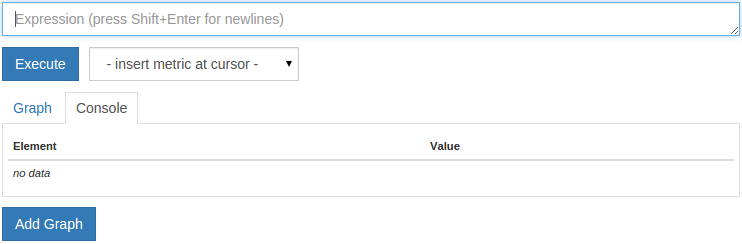
As you can see, there are two tabs: Graph and Console. Prometheus allows you to query data in two different modes:
- The "Console" tab allows you to evaluate the query expression at the current time. After running the query, the table will display the current value of each result time series (one table row per output series).
- The "Graph" tab allows you to draw query expressions within a specified time range.
Since Prometheus can scale to millions of time series, it is possible to build very expensive queries (think of it as similar to selecting all rows from a large table in a SQL database). To avoid queries that time out or overload the server, it is recommended to start exploring and constructing queries in the Console view instead of drawing them immediately. Evaluating a potentially expensive query at a single point in time will have far fewer resources than trying to plot the same query over a period of time.
Once you have sufficiently narrowed the scope of the query (according to the series it chooses to load, the number of calculations it needs to perform, and the number of output time series), you can switch to the Graph tab to display calculation expressions over time. Knowing when the price of a query is cheap enough is not an exact science, it depends on your data, latency requirements, and the capabilities of the machine running the Prometheus server. Over time, you will feel this way.
Since our test Prometheus server does not scrape large amounts of data, we can't actually formulate any costly queries in this tutorial. Any sample query can be viewed in the "Graph" and "Console" views without any risk.
To reduce or increase the graph time range, click the - or + button. To move the end time of the graph, press the << or >> button. You can stack graphics by activating the Stack checkbox. Finally, **Res. (S) **Input allows you to specify a custom query resolution (not required for this tutorial).
Step 4-Perform a simple time series query
Before we start the query, let's quickly review the Prometheus data model and terminology. Prometheus basically stores all data as a time series. Each time series is identified by the metric name and a set of key-value pairs that Prometheus calls label. The metric name indicates the overall aspect of the system being measured (for example, the number of HTTP requests processed since the process started http_requests_total). Labels are used to distinguish sub-dimensions of the measure, such as HTTP method (e.g. method="POST") or path (e.g. path="/api/foo"). Finally, a series of samples form a series of actual data. Each sample consists of a timestamp and a value, where the timestamp has millisecond precision and the value is always a 64-bit floating point value.
The simplest query we can make returns all series with a given metric name. For example, the demo service exports a metric demo_api_request_duration_seconds_count, which represents the number of synthetic API HTTP requests processed by the virtual service. You may wonder why the metric name contains the string duration_seconds. This is because this counter is part of a larger histogram metric. The metric demo_api_request_duration_seconds mainly tracks the distribution of request durations, but also discloses the total count of tracking requests (here with the suffix _count) as Useful by-products.
Make sure the "ConsoleQuery" tab is selected, enter the following query in the text field at the top of the page, and then click the "Execute" button to execute the query:
demo_api_request_duration_seconds_count
Since Prometheus is monitoring three service instances, you should see a tabular output with 27 result time series with this metric name, one for each tracking service instance, path, HTTP method, and HTTP status code. In addition to the service instance itself (setting the labels method, path and status), the series will have appropriate job and instance labels to distinguish different service instances from each other. When storing the time series of scraped targets, Prometheus automatically attaches these tags. The output should look like this:
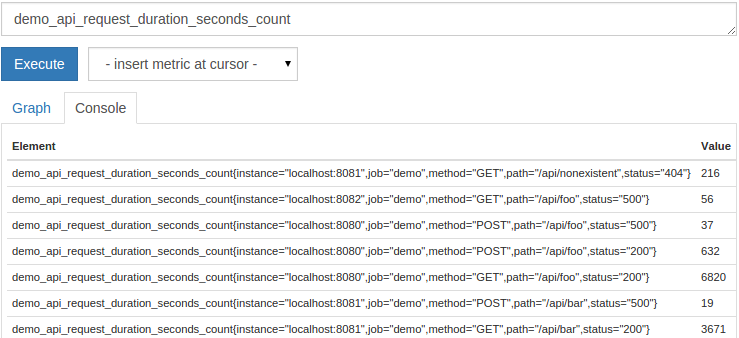
The values displayed in the column on the right are the current values of each time series. You can freely draw the output graph (click the "Graph" tab and click "**Execute" again) to get this query and subsequent queries to see how the value changes over time.
We can now add a tag matcher to limit the returned series based on tags. The tag matcher directly follows the metric name in curly braces. In the simplest form, they filter the series with the exact value of a given label. For example, this query only displays the request count for any GET request:
demo_api_request_duration_seconds_count{method="GET"}
The matcher can use a combination of commas. For example, we can also filter metrics only from the instance localhost:8080 and the job demo:
demo_api_request_duration_seconds_count{instance="localhost:8080",method="GET",job="demo"}
The result will look like this:
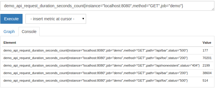
When combining multiple matchers, all matchers need to be matched to select a series. The above expression only returns the API request count of the service instance running on port 8080 and the location of the HTTP method GET. We also make sure to select only indicators that belong to the demo position.
Note: It is recommended to always specify the label job when selecting a time series. This ensures that you will not accidentally choose indicators with the same name from different jobs (unless of course this is indeed your goal!). Although we are only monitoring one job in this tutorial, we will still select by job name in most of the examples below to emphasize the importance of this exercise.
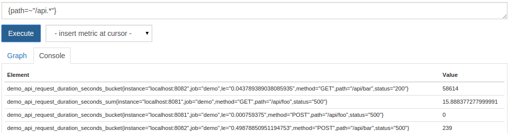
In addition to equal matching, Prometheus also supports non-equal matching (!=), regular expression matching (=~) and negative regular expression matching (!~). You can also omit the metric name completely and use only the tag matcher for query. For example, to list all the series (regardless of the metric name or job) where the path tag starts with /api, you can run this query:
{ path=~"/api.*"}
Since the regular expression ending in .* always matches the complete string in Prometheus, the above regular expression needs to end.
The resulting time series will be a mixture of series with different metric names:
You now know how to select a time series based on the combination of its metric name and their label values.
Step 5-Calculate interest rates and other derivatives
In this section, we will learn how to calculate the rate or increment of a metric.
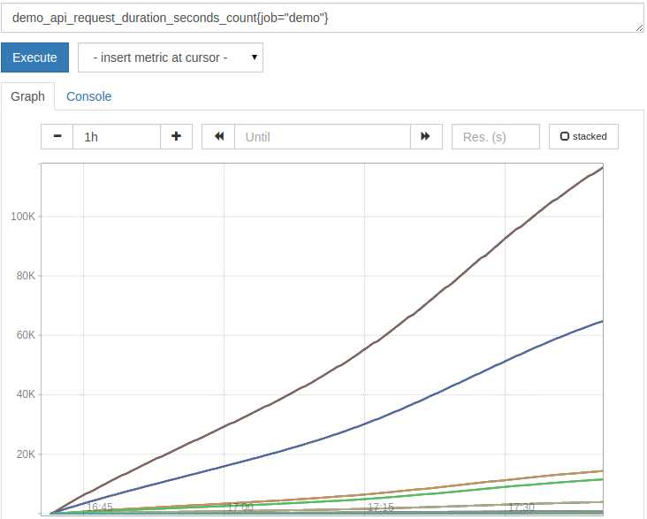
One of the most common functions you will use in Prometheus is rate(). In Prometheus, instead of calculating the event rate directly in the instrumented service, you usually use the original counter to track the event and let the Prometheus server temporarily calculate the rate during the query time (this has many advantages, such as not losing the rate peak. Time, and the ability to select a dynamic average window during query). The counter starts from 0 when the monitored service starts, and continues to increase during the life cycle of the service process. Sometimes, when the monitored process restarts, its counter will be reset to 0 and then start climbing again from there. Plotting raw counters is usually not very useful, because you will only see increasing rows and occasionally reset. You can view it by plotting the API request count of the demo service:
demo_api_request_duration_seconds_count{job="demo"}
It looks a bit like this:
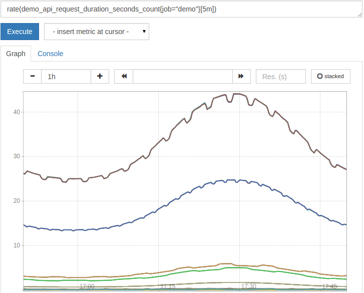
To make counters useful, we can use the rate() function to calculate their per second growth rate. We need to tell rate() to determine the time window of the average rate by providing a range selector after the series matcher (such as [5m]). For example, to calculate the per second increment of the above counter indicator (such as the average of the past five minutes), draw the following query:
rate(demo_api_request_duration_seconds_count{job="demo"}[5m])
The results are now more useful:
rate() is smart and automatically adjusts the counter reset by assuming that any reset of the counter value is a reset.
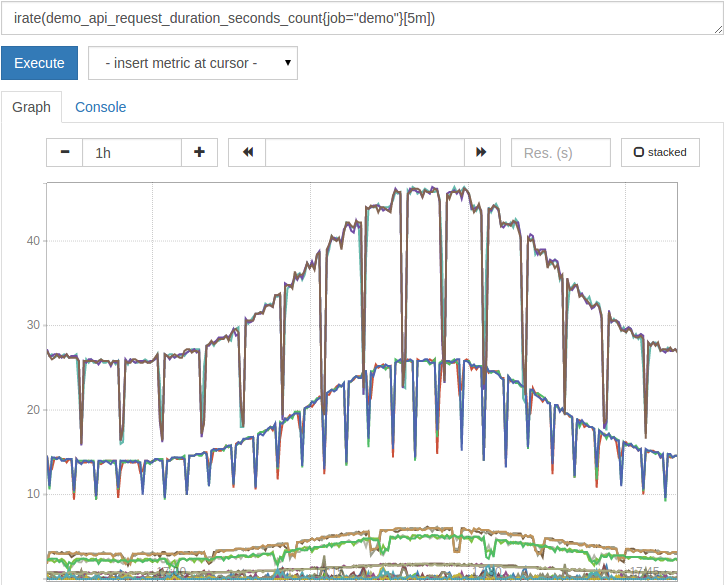
A variant of rate() is irate(). Although rate() averages the rate of all samples within a given time window (5 minutes in this case), irate() can only review the past two samples. It still requires you to specify a time window (such as [5m]) to know the maximum lookback time for these two samples. irate() will react faster to rate changes, so it is usually recommended for graphs. On the contrary, rate() will provide a smoother rate and is recommended for alarm expressions (because short-term peaks will be suppressed and will not wake you up at night).
With irate(), the above chart looks like this, with short intermittent drops in the request rate:
rate() and irate() always calculate the rate per second. Sometimes you want to know the total amount that the counter has increased over a period of time, but you can still correct the reset of the counter. You can use the increase() function for this purpose. For example, to calculate the total number of requests processed in the past hour, please query:
increase(demo_api_request_duration_seconds_count{job="demo"}[1h])
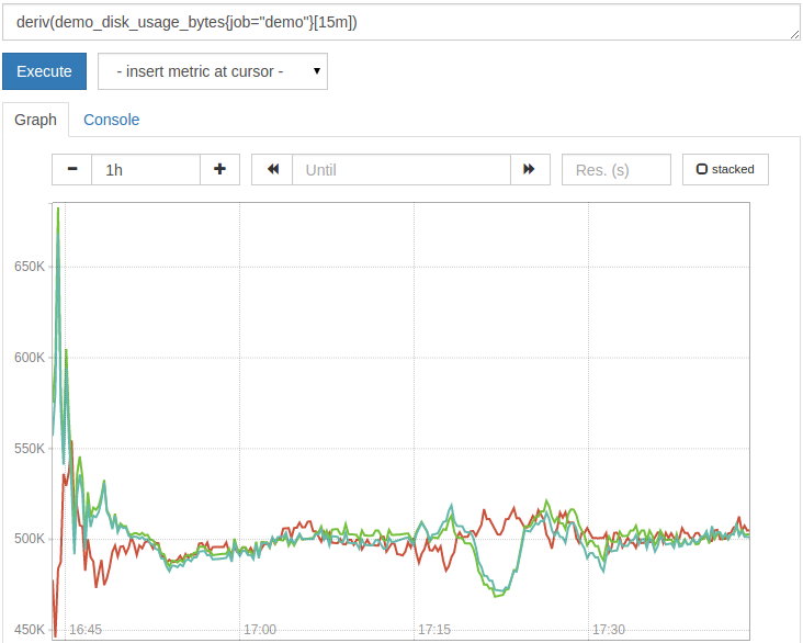
In addition to the counter (which can only be increased), there are also measurement indicators. A meter is a value that can rise or fall over time, such as temperature or available disk space. If we want to calculate the change of the meter over time, we cannot use the rate()/ irate()/ increase() series of functions. These are all for the counter, because they interpret any decrease in the metric value as a counter reset and compensate for it. Instead, we can use the deriv() function, which calculates the derivative per second of the meter based on linear regression.
For example, to see how fast the usage of the fictitious disk exported by our demo service has increased or decreased (in MiB per second) based on the linear regression of the last 15 minutes, we can query:
deriv(demo_disk_usage_bytes{job="demo"}[15m])
The result should look like this:
We now know how to calculate the rate per second with different average behavior, how to handle the counter reset in the rate calculation, and how to calculate the derivative of the meter.
Step 6-Aggregate Time Series
In this section, we will learn how to aggregate a single series.
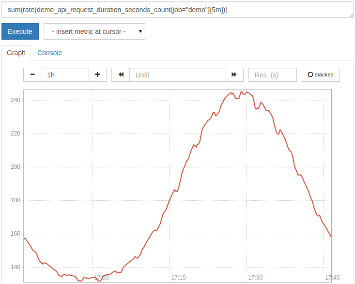
Prometheus collects data with high dimensional details, which can result in many series of each metric name. However, usually you don't care about all sizes, and there may even be too many series to draw them all at once in a reasonable way. The solution is to aggregate certain dimensions and keep only the dimensions you care about. For example, the demo service traces API HTTP requests method, path and status. When Prometheus scraped from node exporters, it added a further dimension: where did the metrics instance and job come from for tracking label processing. Now, to see the total request rate of all dimensions, we can use the sum() aggregation operator:
sum(rate(demo_api_request_duration_seconds_count{job="demo"}[5m]))
However, this aggregates all dimensions and creates a single output series:
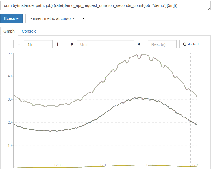
But usually, you need to keep some dimensions in the output. For this reason, sum() and other aggregators support a without( <label names>) clause that specifies the dimensions to be aggregated. There is also an alternative reverse by(</label> <label names>) clause that allows you to specify the label name to keep. If we want to know the total request rate summed across all three service instances and all paths, but split the result by method and status code, we can query:
sum without(method, status)(rate(demo_api_request_duration_seconds_count{job="demo"}[5m]))
This is equivalent to:
sum by(instance, path, job)(rate(demo_api_request_duration_seconds_count{job="demo"}[5m]))
The result is now grouped by instance, path and job:
**Note **: Always calculate rate(), irate() or increase() before apply any aggregation. If you apply aggregation first, it will hide the counter reset and these functions will no longer work properly.
Prometheus supports the following aggregation operators, each of which supports a by() or without() clause to select the dimensions to keep:
sum: Summarize all values in the aggregation group.min: Select the minimum value of all values in the aggregation group.max: Select the maximum value of all values in the aggregation group.avg: Calculate the average (arithmetic average) of all values in the aggregation group.stddev: Calculate the standard deviation of all values in the aggregation group.stdvar: Calculate the standard difference of all values in the aggregation group.count: Calculate the total number of sequences in the aggregation group.
You have now learned how to aggregate a list of series and how to keep only the dimensions you care about.
Step 7-Perform arithmetic
In this section, we will learn how to perform arithmetic operations in Prometheus.
As the simplest arithmetic example, you can use Prometheus as a number calculator. For example, run the following query in the "Console" view:
(4+7)*3
You will get a single scalar output value 33:
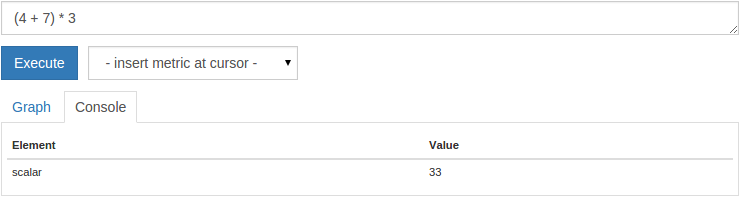
Scalar values are simple numbers without any labels. To make this more useful, Prometheus can apply ordinary arithmetic operators (+, -, *, /, %) to the entire time series vector. For example, the following query converts the simulated processing bytes of the last batch job run into MiB:
demo_batch_last_run_processed_bytes{job="demo"}/1024/1024
The result will be displayed in MiB:
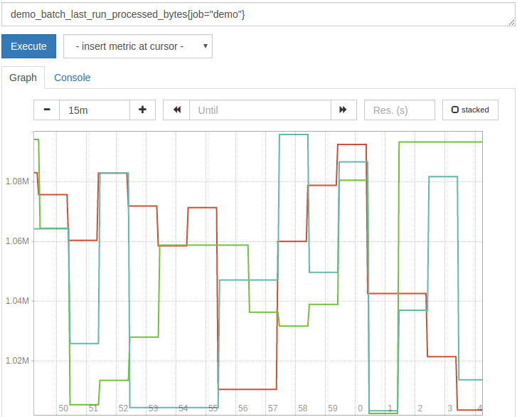
Although good visualization tools (such as Grafana) can also handle the conversion for you, simple algorithms are often used for these types of unit conversions.
The feature of Prometheus (where Prometheus really shines!) is the binary arithmetic between two sets of time series. When using binary operators between two sets of series, Prometheus will automatically match elements with the same label set on the left and right sides of the operation, and apply the operator to each matched pair to generate an output sequence.
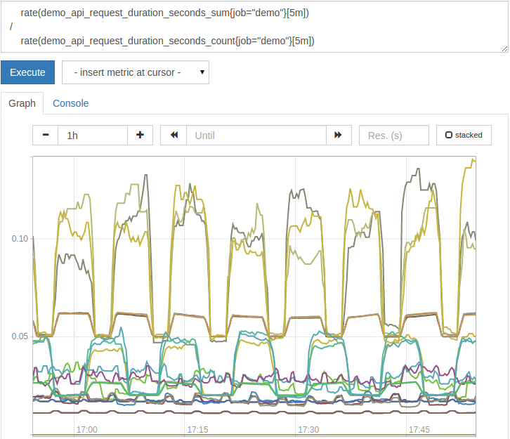
For example, the demo_api_request_duration_seconds_sum metric tells us how many seconds it took to answer an HTTP request, while demo_api_request_duration_seconds_count tells us how many HTTP requests. The two indicators have the same size (method, path, status, instance, job). To calculate the average request latency for each dimension, we can simply query the ratio of the total time spent in the request divided by the total number of requests.
rate(demo_api_request_duration_seconds_sum{job="demo"}[5m])/rate(demo_api_request_duration_seconds_count{job="demo"}[5m])
Please note that we also wrap a rate() function on each side of the operation to only consider the delay of requests that occurred in the last 5 minutes. This also increases the flexibility to resist counter resets.
The resulting average request latency graph should look like this:
But what should we do when the tags do not match exactly on both sides? This happens especially when we have time series sets of different sizes on both sides of the operation, because the size on one side is larger than the size on the other side. For example, the demo job export spends fictitious CPU time (idle, user, system) in various modes as the indicator demo_cpu_usage_seconds_total with the size of the mode tag. It will also export a fictitious total CPU as demo_num_cpus (this indicator has no additional dimensions). If you try to divide one by the other to reach the average CPU usage percentage of each of the three modes, the query will not produce any output:
# BAD!
 # Multiply by 100 to getfrom a ratio to a percentage
 rate(demo_cpu_usage_seconds_total{job="demo"}[5m])*100/
 demo_num_cpus{job="demo"}
In these one-to-many or many-to-one matching, we need to tell Prometheus which subset of tags to use for matching, and we also need to specify how to handle additional dimensions. In order to solve the matching problem, we added an on( <label names>) clause to the binary operator
In this case, the correct query would be:
 # Multiply by 100 to getfrom a ratio to a percentage
 rate(demo_cpu_usage_seconds_total{job="demo"}[5m])*100/on(job, instance)group_left(mode)
 demo_num_cpus{job="demo"}
The result should look like this:
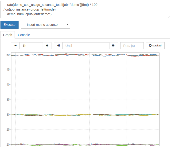
The on(job, instance) tells the operator to only match the series from the left and right on its job and instance labels (and therefore not on the mode label, which is incorrect on the right Exist), and the group_left(mode) clause tells the operator to fan out and display the average CPU usage of each mode. This is the case of many-to-one matching. To perform reverse (one-to-many) matching, use the group_right( <label names>) clause in the same way
You now know how to use arithmetic between sets of time series and how to handle different dimensions.
in conclusion
In this tutorial, we set up a set of demo service instances and monitor them using Prometheus. Then, we learned how to apply various query techniques to the collected data to answer the questions we care about. You now know how to select and filter series, how to aggregate sizes, and how to calculate rates or derivatives or do arithmetic. You also learned how to structure queries in general and how to avoid overloading the Prometheus server.
To learn more about querying Prometheus related tutorials, please go to Tencent Cloud + Community to learn more.
Reference: "How To Query Prometheus on Ubuntu 14.04 Part 1"
Recommended Posts