How to query Prometheus on Ubuntu 14.04 part 2
Introduction
Prometheus is an open source monitoring system and time series database. In How to Query Prometheus in Ubuntu 14.04 Part 1, we set up three demonstration service instances to expose synthetic metrics to the Prometheus server. Using these indicators, we learned how to use the Prometheus query language to select and filter time series, how to aggregate dimensions, and how to calculate rates and derivatives.
In the second part of this tutorial, we will build the settings from the first part and learn more advanced query techniques and patterns. After this tutorial, you will learn how to apply value-based filtering, set operations, histograms, etc.
To complete this tutorial, you need to have an Ubuntu server with a non-root account that can be used with the sudo command, and the firewall is turned on. Students who don’t have a server can buy it from here, but I personally recommend you to use the free Tencent Cloud Developer Lab for experimentation, and then buy server.
Preparation
This tutorial is based on how to query the settings outlined in Prometheus on Ubuntu 14.04 Part 1. At the very least, you need to follow steps 1 and 2 in the tutorial to set up the Prometheus server and three monitored demonstration service instances. However, we will also build on the query language technology explained in the first part, so it is recommended to use it completely.
**Step 1-Filter by value and use threshold **
In this section, we will learn how to filter the returned time series based on its value.
The most common use for value-based filtering is simple digital alarm thresholds. For example, we might want to find HTTP paths with a total 500-status request rate higher than 0.2 per second, which is an average over the past 15 minutes. To do this, we only need to query all 500-status request rates, and then append a filter operator > 0.2 to the end of the expression:
rate(demo_api_request_duration_seconds_count{status="500",job="demo"}[15m])>0.2
In the Console view, the result should look like this:

However, like binary algorithms, Prometheus not only supports filtering by a single scalar number. You can also filter a set of time series based on another set of series. Similarly, elements are matched by their set of tags, and filter operators are applied between matched elements. Only the elements on the left that match the elements on the right * and * pass through the filter become part of the output. on(<labels> ), group_left(<labels> ), group_right(<labels> The ) clause works here in the same way as the arithmetic operators.
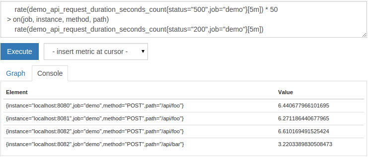
For example, we can choose the 500-status rate for any combination of job, instance, method, and path, and the 200-status rate is not higher than at least 50 times 500-status Rate, like this:
rate(demo_api_request_duration_seconds_count{status="500",job="demo"}[5m])*50>on(job, instance, method, path)rate(demo_api_request_duration_seconds_count{status="200",job="demo"}[5m])
This will look like this:
In addition to >, prometheus also supports the usual >=, <=, <, !=, and == comparison operators for filtering purposes.
We now know how to filter a set of time series based on a single value or based on another set of time series values with matching labels.
**Step 2-Use set operators **
In this section, you will learn how to use Prometheus' set operators to correlate time series sets.
Usually, you want to filter a set of time series based on another set. To this end, Prometheus provides the and set operator. For each series on the left of the operator, it will try to find the series with the same label on the right. If a match is found, the left series becomes part of the output. If there is no matching series on the right, the series is omitted from the output.
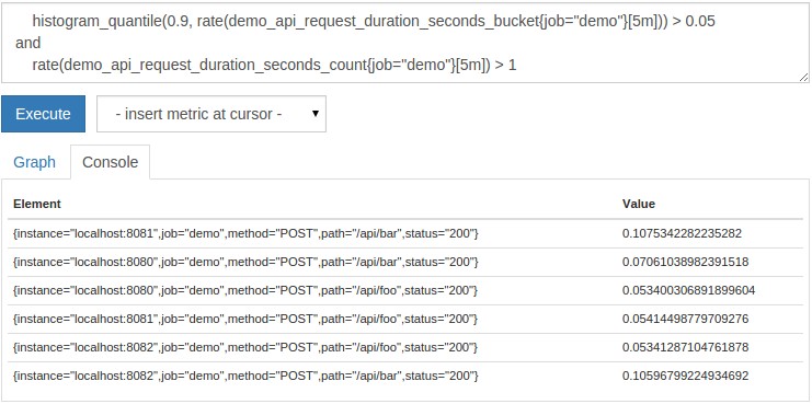
For example, you may wish to choose any HTTP endpoint with a 90% latency higher than 50 milliseconds (0.05 seconds), but limited to a combination of dimensions that receive multiple requests per second. We will use the histogram_quantile() function to calculate percentiles here. We will explain the exact role of this feature in the next section. Currently, it only calculates the 90th percentile delay for each sub-dimension. To filter the error delay caused and only keep the delay of receiving multiple requests per second, we can query:
histogram_quantile(0.9,rate(demo_api_request_duration_seconds_bucket{job="demo"}[5m]))>0.05
and
 rate(demo_api_request_duration_seconds_count{job="demo"}[5m])>1
Sometimes you want to construct a union from two sets of time series instead of using intersection. Prometheus provides the set operator or for this purpose. It results in the left series of the operation, and any left series on the right that does not have a matching label set. For example, to list all request rates below 10 or above 30, please query:
rate(demo_api_request_duration_seconds_count{job="demo"}[5m])<10
or
 rate(demo_api_request_duration_seconds_count{job="demo"}[5m])>30
The results will be displayed in the chart as follows:
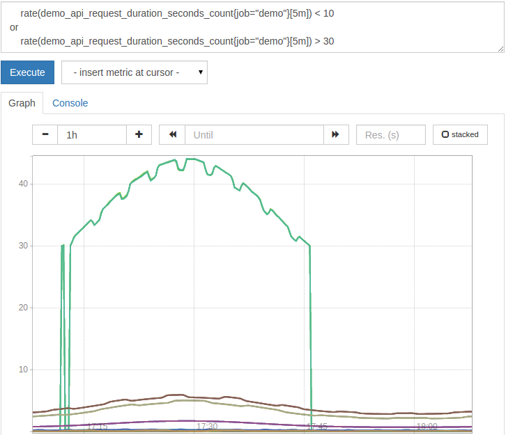
As you can see, using value filters and setting actions in a chart can cause time series to appear and disappear in the same chart, depending on whether they match any time steps in the chart. Generally, it is recommended to only use this type of filter logic for alert rules.
You now know how to construct intersections and unions using labeled time series.
Step 3-Use the histogram
In this section, we will learn how to interpret histogram metrics and how to calculate quantiles (the general form of percentiles) from them.
Prometheus supports histogram indicators, allowing the service to record the distribution of a series of values. Histograms usually track measurements such as request delay or response size, but can fundamentally track any value that fluctuates in amplitude according to a certain distribution. Prometheus histograms sample the data on the client side, which means that they use many configurable (for example, delayed) storage areas to calculate observations, and then expose these storage buckets as separate time series.
Internally, the histogram is implemented as a set of time series, each time series represents the count of a given bucket (for example, "requests under 10ms", "requests under 25ms", "requests under 50ms", etc.). The bucket counter is cumulative, which means that the larger value bucket includes the count of all lower value buckets. On each time series that is part of the histogram, the corresponding bucket is indicated by a special le (less than or equal to) label. This will add additional dimensions to any existing dimensions you have tracked.
For example, our demo service exports a histogram demo_api_request_duration_seconds_bucket that tracks the distribution of API request duration. Since this histogram derives 26 buckets for each tracked sub-dimension, this indicator has a large number of time series. Let us first view the original histogram of a type of request from an example:
demo_api_request_duration_seconds_bucket{instance="localhost:8080",method="POST",path="/api/bar",status="200",job="demo"}
You should see 26 series, each series represents an observation bucket, identified by the label le:

The histogram can help you answer questions such as "How many of my requests require more than 100 milliseconds to complete?" (If the histogram is configured with a bucket with a 100ms boundary). On the other hand, you often want to answer a related question, such as "What is the delay for 99% of the query completion?". If your histogram bucket is fine enough, you can use the histogram_quantile() function to calculate it. This function requires histogram metrics (a set of series with le bucket labels) as its input and outputs the corresponding quantile. In the comparison percentage, its range is from the 0th to the 100th percentile, that is, the target digit specification histogram_quantile() function expects as the input range from 0 to 1 (so the 90th percentile The quantile will correspond to the quantile 0.9).
For example, we can try to calculate the 90% percentile API latency of all dimensions as follows:
# BAD!histogram_quantile(0.9, demo_api_request_duration_seconds_bucket{job="demo"})
This is not very useful or reliable. When a single service instance is restarted, the bucket counter is reset, and you usually want to see the "now" delay (for example, measured in the past 5 minutes) instead of the entire time of the indicator. You can achieve this by applying the rate() function to the basic histogram bucket counters, which both handle counter resets and only consider the rate of increase of each bucket within a specified time window.
Calculate 90% of the API latency in the past 5 minutes as follows:
# GOOD!histogram_quantile(0.9,rate(demo_api_request_duration_seconds_bucket{job="demo"}[5m]))
This is much better, it looks like this:

However, this accounts for each of the sub-dimensions (job, instance, path, method, and status) of your 90th percentile *. Similarly, we may not be interested in all these dimensions and want to aggregate some of them together. Fortunately, the sum aggregation operator of Prometheus can be combined with the histogram_quantile() function to allow us to aggregate dimensions in query time!
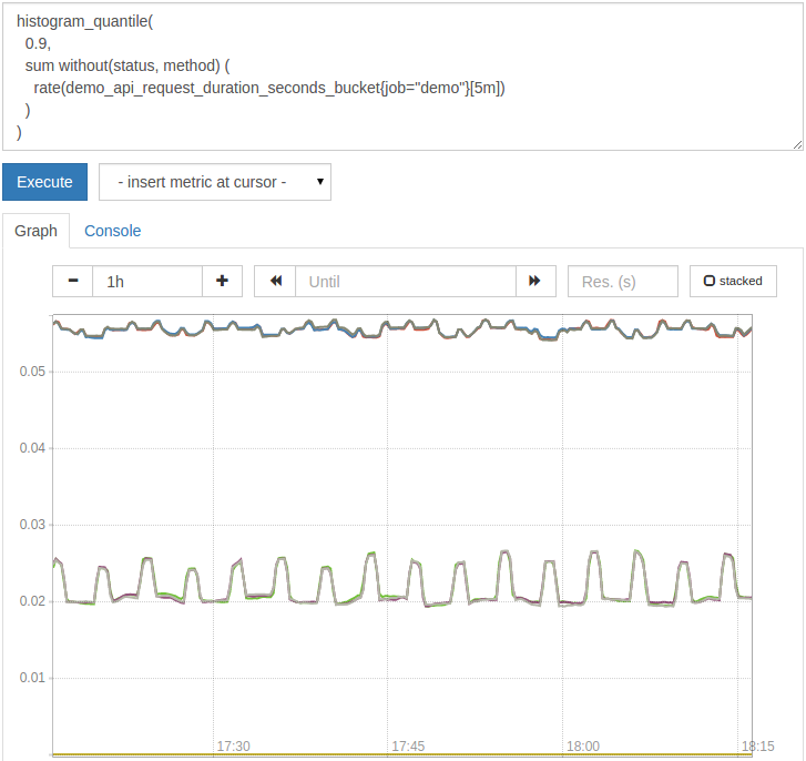
The following query calculates the 90th percentile delay, but can only split the result by the size of job, instance and path:
histogram_quantile(0.9,
 sum without(status, method)(rate(demo_api_request_duration_seconds_bucket{job="demo"}[5m])))
Note: le always keeps the bucket label in any aggregation before applying the histogram_quantile() function. This ensures that it can still operate on the bucket group and calculate the quantile from it.
The diagram now looks like this:
Calculating the quantile from the histogram always introduces a certain amount of statistical error. This error depends on your bucket size, the distribution of observations, and the target quantile you want to calculate.
You now know how to interpret histogram measures and how to calculate quantiles from them in different time frames, and you can also dynamically aggregate certain dimensions.
Step 4-Use Timestamp Indicators
In this section, we will learn how to use metrics that include timestamps.
Components in the prometheus ecosystem often expose timestamps. For example, this might be the last time the batch job completed successfully, the last time the configuration file was successfully reloaded, or the computer was booted. By convention, time is expressed as a Unix timestamp (in seconds) since UTC on January 1, 1970.
For example, the demo service exposes the last successful simulation batch job:
demo_batch_last_success_timestamp_seconds{job="demo"}
This batch job was simulated to run every minute, but failed in 25% of all attempts. In the case of failure, the demo_batch_last_success_timestamp_seconds metric maintains its last value until another successful run occurs.
If you draw the original timestamp graph, it will look like this:
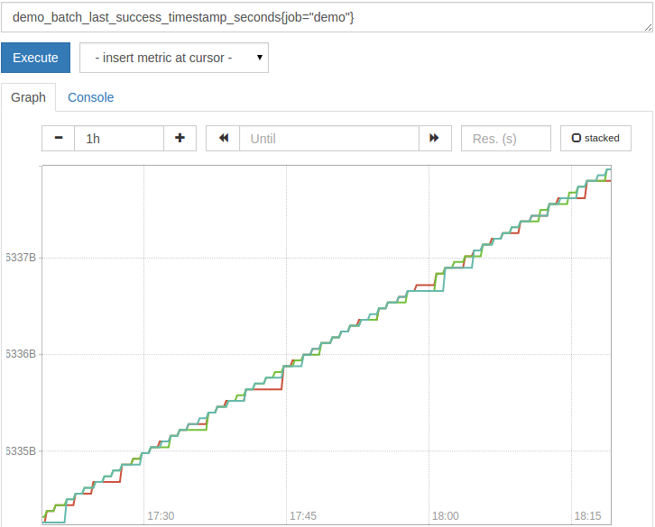
As you can see, the original timestamp value itself is usually not very useful. Instead, you often want to know the age of the timestamp value. A common pattern is to subtract the timestamp in the measurement from the current time, as provided by the time() function:
time()- demo_batch_last_success_timestamp_seconds{job="demo"}
This will produce the number of seconds since the last successful run of the batch job:

If you want to convert this age from seconds to hours, you can divide the result by 3600:
( time()- demo_batch_last_success_timestamp_seconds{job="demo"})/3600
Expressions like this are useful for drawing and alerting. When visualizing the timestamp age as above, you will receive a sawtooth graph with linearly increasing rows and periodically reset to 0 when the batch job is successfully completed. If the saw-tooth spike becomes too large, it means that the batch job has not been completed for a long time. You can also alert you by adding a threshold filter to the > expression and alerting the generated time series (although we won't introduce the alert rules in this tutorial).
To simply list the instances where the batch job has not completed in the last 1.5 minutes, you can run the following query:
time()- demo_batch_last_success_timestamp_seconds{job="demo"}>1.5*60
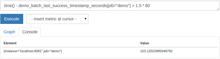
You now know how to convert raw timestamp metrics to relative age, which is helpful for graphs and alerts.
Step 5-Sort and use topk/bottomk functions
In this step, you will learn how to sort the query output or select only the maximum or minimum of a set of series.
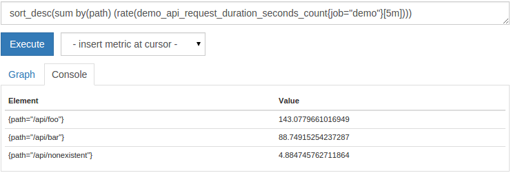
In the table console view, it is often useful to sort the output series by the value of the output series. You can use the sort() (ascending order) and sort_desc() (descending order) functions to achieve this. For example, to display the request rate of each route sorted by its value, from highest to lowest, you can query:
sort_desc(sum by(path)(rate(demo_api_request_duration_seconds_count{job="demo"}[5m])))
The sorted output is as follows:
Or you may not be interested in showing all the series at all, but only the series with the largest or smallest K. To this end, prometheus provides topk() and bottomk() functions. They each take a K value (how many series to choose) and an arbitrary expression, which returns a set of time series that should be filtered. For example, to display only the first three request rates for each path and method, you can query:
topk(3, sum by(path, method)(rate(demo_api_request_duration_seconds_count{job="demo"}[5m])))
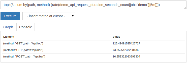
While the sorting is only useful in the console view, topk() and bottomk() can also be useful in graphs. Note that the output will not show the top or bottom K series averaged over the entire graph time range-instead, the output will recalculate the K top or bottom output series for each resolution step in the graph. Therefore, your top or bottom K series can actually vary within the range of the chart, and your chart may show more than the K series in total.
We have now learned how to sort or select only the series with the largest or smallest K.
Step 6-Check the health of the scraped instance
In this step, we will learn how to check the scratch health of an instance over time.
To make this part more interesting, let's terminate the first of your three background demo service instances (listening on port 8080):
pkill -f ---listen-address=:8080
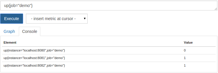
Whenever prometheus scratches the target, it will store the composite sample up with the metric name and the label of the instance scraped off with job and instance. If the scraping is successful, set the value of the sample to 1. If the scraping fails, set to 0. Therefore, we can easily query the current "up" or "down" instance:
up{job="demo"}
An instance should now be displayed as down:
To only show down instances, you can filter the value 0:
up{job="demo"}==0
You should now only see the instance you terminated:

Or, to get the total number of closed instances:
count by(job)(up{job="demo"}==0)
This will display 1:

These types of queries are useful for basic scratch health alerts.
Note: If the instance is not closed, this query will return an empty result instead of a single output series with a count of 0. This is because the count() aggregation operator requires a set of dimensional time series as its input, and the output sequence can be grouped according to the by or without clause. Any output group can only be based on an existing input series-if there is no input series at all, no output will be produced.
You now know how to query the health status of an instance.
in conclusion
In this tutorial, we have constructed how to query the progress of Prometheus on Ubuntu 14.04 Part 1, and introduced more advanced query techniques and patterns. We learned how to filter series based on the value of the series, calculate quantiles from histograms, deal with timestamp-based indicators, etc.
Although these tutorials cannot cover all possible query use cases, we hope that the example queries will be useful to you when using Prometheus to build actual queries, dashboards, and alerts.
To learn more about querying Prometheus related tutorials, please go to [Tencent Cloud + Community] (https://cloud.tencent.com/developer?from=10680) to learn more.
Reference: "How To Query Prometheus on Ubuntu 14.04 Part 2"
Recommended Posts