9 feature engineering techniques of Python

The code attached to this article can be found here.
https://github.com/NMZivkovic/top_9_feature_engineering_techniques
In this article, the most effective element engineering techniques usually required to obtain good results are explored.
Don't get me wrong, functional design is not just to optimize the model. Sometimes it is necessary to apply these techniques so that the data is compatible with machine learning algorithms. Machine learning algorithms sometimes expect to format data in a certain way, and this is where feature engineering can help. In addition, it should be noted that data scientists and engineers spend most of their time on data preprocessing. This is why it is important to master these technologies. Explore in this article:
- Attribution
- Classification code
- Handling outliers
- Boxing
- scaling ratio
- Log conversion
- Function selection
- Function grouping
- Functional split
Data set and prerequisites
For the purposes of this tutorial, make sure you have installed the following Python libraries:
- NumPy
- SciKit Learn
- Pandas
- Matplotlib
- SeaBorn
After the installation is complete, make sure you have imported all the necessary modules used in this tutorial.
import pandas as pd
import numpy as np
import matplotlib.pyplot as plt
import seaborn as sb

from sklearn.preprocessing import StandardScaler, MinMaxScaler, MaxAbsScaler, QuantileTransformer
from sklearn.feature_selection import SelectKBest, f_classif
The data used in this article comes from the PalmerPenguins dataset. This data set was recently introduced to replace the famous Iris data set. It was created by Dr. Kristen Gorman and Palmer Station in Antarctica. You can get this dataset here or through Kaggle. This data set essentially consists of two data sets, each of which contains data for 344 penguins. Just like in the iris data set, there are 3 different penguins in the 3 islands of the Palmer Islands.
https://github.com/allisonhorst/palmerpenguins
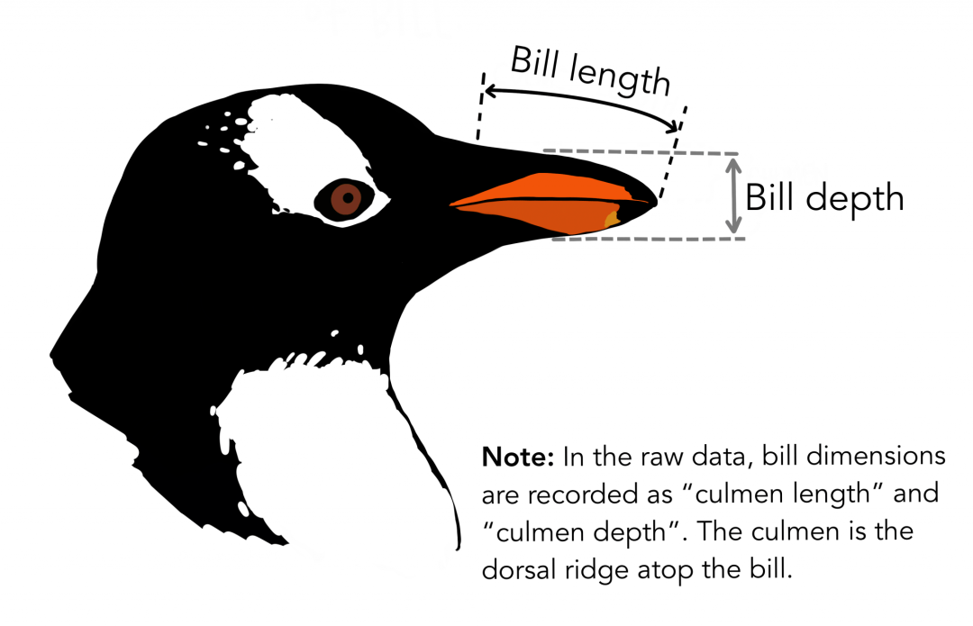
Again, these data sets contain specimen dimensions for each species. The high gate is the upper ridge of the beak. In the simplified penguin data, the vertex length and depth have been renamed to the culmen_length_mm and culmen_depth_mm variables. Use Pandas to load this dataset:
data = pd.read_csv('./data/penguins_size.csv')
data.head()
1. Attribution
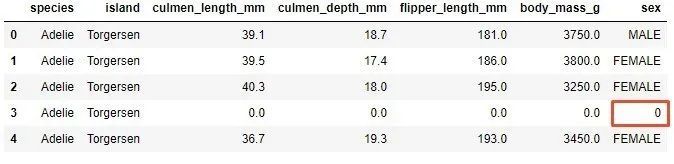
The data obtained from customers can take various forms. Usually it is sparse, which means that some samples may lack data for certain functions. Need to detect these instances and delete these samples, or replace the null value with some value. Depending on the rest of the data set, different strategies may be applied to replace those missing values. For example, these empty slots can be filled with average or maximum eigenvalues. But first detect the missing data. You can use Pandas for this:
print(data.isnull().sum())
-
species 0*
-
island 0*
-
culmen_length_mm 2*
-
culmen_depth_mm 2*
-
flipper_length_mm 2*
-
body_mass_g 2*
-
sex 10*
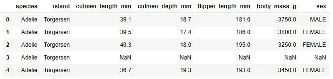
This means that there are instances in the dataset that lack values for certain elements. Two instances lack the culmen_length_mm feature value, and 10 instances lack the gender feature. You can even see in the first few examples (NaN means not a number, which means missing value):
The easiest way to deal with missing values is to delete samples with missing values from the data set. In fact, some machine learning platforms will automatically do this for you. However, due to the reduced data set, this may reduce the performance of the data set. Using Pandas again is the easiest way:
data = pd.read_csv('./data/penguins_size.csv')
data = data.dropna()
data.head()
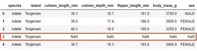
Note that the third sample with missing values has been removed from the data set. This is not the best choice, but it is sometimes necessary because most machine learning algorithms are not suitable for sparse data. Another method is to use imputation, which is to replace missing values. To do this, you can pick some values, or use average eigenvalues, or average eigenvalues. And you must be careful. Observe the missing value in the row at index 3:
If you replace it with simple values only, the same value will be applied for categorical and numerical features:
data = data.fillna(0)

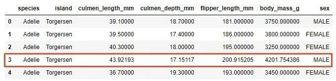
Missing data was detected in the digital features culmen_length_mm, culmen_depth_mm, flipper_length_mm and body_mass_g. For the estimated values of these features, the average value of the features will be used. For the classification feature of "sex", the most frequent value is used. This is the method:
data = pd.read_csv('./data/penguins_size.csv')

data['culmen_length_mm'].fillna((data['culmen_length_mm'].mean()), inplace=True)
data['culmen_depth_mm'].fillna((data['culmen_depth_mm'].mean()), inplace=True)
data['flipper_length_mm'].fillna((data['flipper_length_mm'].mean()), inplace=True)
data['body_mass_g'].fillna((data['body_mass_g'].mean()), inplace=True)

data['sex'].fillna((data['sex'].value_counts().index[0]), inplace=True)

data.reset_index()
data.head()
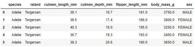
Observe what the third example mentioned looks like now:
Usually the data will not be lost, but its value is invalid. For example, know that for the "gender" function, there can be two values: FEMALE and MALE. You can check if there are other values:
data.loc[(data['sex']!='FEMALE')&(data['sex']!='MALE')]
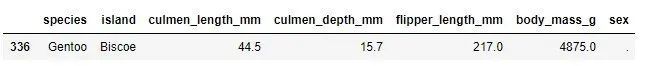
It turns out that there is a record with the value ".". For this function, this is incorrect. You can treat these instances as lost data and discard or replace them:
data = data.drop([336])
data.reset_index()
2. Classification code
One way to improve prediction is to use clever methods when dealing with categorical variables. As the name suggests, these variables have discrete values and represent a certain category or category. For example, the color can be a categorical variable ("red", "blue", "green"). The challenge is to include these variables in data analysis and use them with machine learning algorithms. Some machine learning algorithms can support categorical variables without further manipulation, but some cannot. This is why we use classification codes. In this tutorial, several types of classification codes are introduced, but before proceeding, let’s extract the conversion of these variables in the dataset into individual variables and mark them as classification types:
data["species"]= data["species"].astype('category')
data["island"]= data["island"].astype('category')
data["sex"]= data["sex"].astype('category')
data.dtypes
-
species category*
-
island category*
-
culmen_length_mm float64*
-
culmen_depth_mm float64*
-
flipper_length_mm float64*
-
body_mass_g float64*
-
sex category*
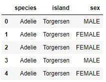
categorical_data = data.drop(['culmen_length_mm','culmen_depth_mm','flipper_length_mm', \
  ' body_mass_g'], axis=1)
categorical_data.head()
Okay, now we can start. Start with the simplest coding label coding.
2.1 Label coding
The label encoding converts each categorical value into some numbers. For example, the "species" function contains 3 categories. You can assign the value 0 to Adelie, 1 to Gentoo, and 2 to Chinstrap. To perform this technique, we can use Pandas:
categorical_data["species_cat"]= categorical_data["species"].cat.codes
categorical_data["island_cat"]= categorical_data["island"].cat.codes
categorical_data["sex_cat"]= categorical_data["sex"].cat.codes
categorical_data.head()
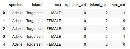
As you can see, three new functions have been added, each of which contains a coded classification function. From the first five examples, we can see that the code value of species category Adelie is 0, the code value of island category Torgensn is 2, and the code value of sex categories FEMALE and MALE are 0 and 1, respectively.
2.2 One-click coding
This is one of the most popular classification coding techniques. It spreads the value in one feature to multiple flag features and assigns a value of 0 or 1. The binary value represents the relationship between uncoded and coded features.

For example, in the data set, there are two possible values in the "sex" function: FEMALE and MALE. The technology will create two separate functions, labeled "sex_female" and "sex_male". If in the "sex" feature, there is a value "female as some samples", "sex_female" will be assigned the value 1 and "sex_male" will be assigned the value 0. Similarly, if in the feature of "sex", for some samples, the value "MALE" will be assigned a value of 1 for "sex_male" and a value of 0 for "sex_female"' will be assigned. Apply this technique to classified data and see what you get:
encoded_spicies = pd.get_dummies(categorical_data['species'])
encoded_island = pd.get_dummies(categorical_data['island'])
encoded_sex = pd.get_dummies(categorical_data['sex'])

categorical_data = categorical_data.join(encoded_spicies)
categorical_data = categorical_data.join(encoded_island)
categorical_data = categorical_data.join(encoded_sex)
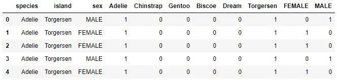
When adding some new columns here. In essence, each category in each function has a separate column. Usually only a hot coded value is used as the input of the machine learning algorithm.
2.3 Counting code
Count coding converts each categorical value into its frequency, that is, the number of times it appears in the data set. For example, if the "species" function contains 6 occurrences of the Adelie class, each Adelie value will be replaced with the number 6. This is how it works in the code:
categorical_data = data.drop(['culmen_length_mm','culmen_depth_mm', \
  ' flipper_length_mm','body_mass_g'], axis=1)

species_count = categorical_data['species'].value_counts()
island_count = categorical_data['island'].value_counts()
sex_count = categorical_data['sex'].value_counts()

categorical_data['species_count_enc']= categorical_data['species'].map(species_count)
categorical_data['island_count_enc']= categorical_data['island'].map(island_count)
categorical_data['sex_count_enc']= categorical_data['sex'].map(sex_count)

categorical_data
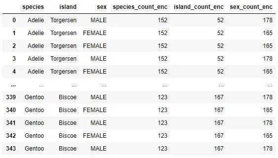
Note how to replace each category value with the number of occurrences.
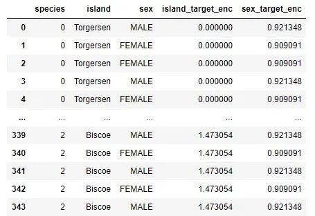
2.4 Target encoding
Unlike the previous technology, this technology is slightly more complicated. It replaces the output averaged with a categorical value (ie, target) as the value of the feature. Essentially what needs to be done is to calculate the average output of all rows with a specific category value. Now when the output value is a number, this is very simple. If the output is classified, for example in the PalmerPenguins data set, some previous techniques need to be applied to it.

Usually, this average value is mixed with the outcome probability of the entire data set to reduce the variance of values that occur rarely. It is important to note that since the category value is calculated based on the output value, these calculations should be performed on the training data set and then applied to other data sets. Otherwise, you will face information leakage, which means that information about the output value of the test set will be included in the training set. This will invalidate the test or give false confidence. Good look at how to do this in code:
categorical_data["species"]= categorical_data["species"].cat.codes

island_means = categorical_data.groupby('island')['species'].mean()
sex_means = categorical_data.groupby('sex')['species'].mean()
Here, the label encoding is used for the output features, and then the average value is calculated for the classification features "island" and "gender". This is the understanding of the "island" function:
island_means
-
island*
-
Biscoe 1.473054*
-
Dream 0.548387*
-
Torgersen 0.000000*
This means that the values Biscoe, Dream and Torgersen will be replaced with the values 1.473054, 0.548387 and 0 respectively. For the "gender" function, we have a similar situation:
sex_means
-
sex*
-
FEMALE 0.909091*
-
MALE 0.921348*
This means that the values FEMALE and MALE will be replaced with 0.909091 and 0.921348 respectively. This is what the data set looks like:
categorical_data['island_target_enc']= categorical_data['island'].map(island_means)
categorical_data['sex_target_enc']= categorical_data['sex'].map(sex_means)
categorical_data
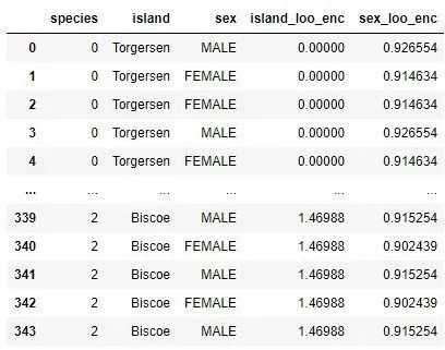
2.5 Keep target code
The final encoding type discussed in this tutorial is based on the target encoding. It works in the same way as the target encoding, but it is different. When calculating the average output value of a sample, exclude the sample. This is how it is done in code. First define a function to perform this operation:
def leave_one_out_mean(series):
series =(series.sum()- series)/(len(series)-1)return series
Then, apply it to the classification value in the dataset:
categorical_data['island_loo_enc']= categorical_data.groupby('island')['species'].apply(leave_one_out_mean)
categorical_data['sex_loo_enc']= categorical_data.groupby('sex')['species'].apply(leave_one_out_mean)
categorical_data
3. Handling outliers
Outliers are values that deviate from the overall distribution of the data. Sometimes these values are wrong and wrong measures and should be removed from the data set, but sometimes they are valuable edge case information. This means that sometimes we want to keep these values in the data set because they may contain some important information, while other times, due to information errors, we want to delete these samples.
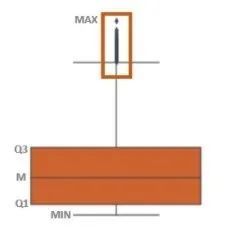
In short, the interquartile range can be used to detect these points. The interquartile range or IQR indicates where 50% of the data is located. When looking for this value, we first look for the median, because it splits the data in half. Then locate the median of the low end of the data (denoted as Q1) and the median of the high end of the data (denoted as Q3). The data between Q1 and Q3 is IQR. Outliers are defined as samples below Q1 – 1.5 (IQR) or above Q3 + 1.5 (IQR). You can use box plots. The purpose of the box plot is to visualize the distribution. Essentially, it includes important points: maximum, minimum, median and two IQR points (Q1, Q3). The following is an example of a box plot:
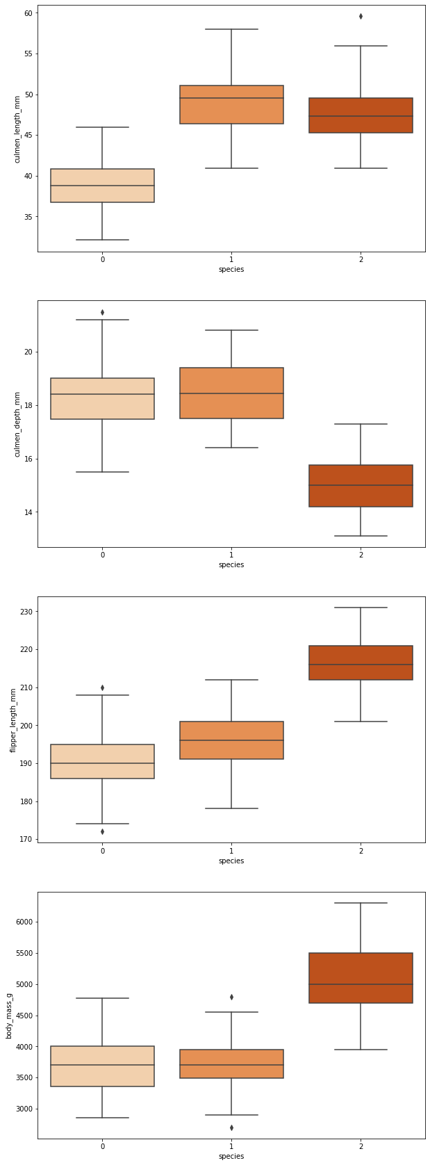
Apply it to the PalmerPenguins dataset:
fig, axes = plt.subplots(nrows=4,ncols=1)
fig.set_size_inches(10,30)
sb.boxplot(data=data,y="culmen_length_mm",x="species",orient="v",ax=axes[0], palette="Oranges")
sb.boxplot(data=data,y="culmen_depth_mm",x="species",orient="v",ax=axes[1], palette="Oranges")
sb.boxplot(data=data,y="flipper_length_mm",x="species",orient="v",ax=axes[2], palette="Oranges")
sb.boxplot(data=data,y="body_mass_g",x="species",orient="v",ax=axes[3], palette="Oranges")
Another way to detect and eliminate outliers is to use standard deviation.
factor =2
upper_lim = data['culmen_length_mm'].mean()+ data['culmen_length_mm'].std()* factor
lower_lim = data['culmen_length_mm'].mean()- data['culmen_length_mm'].std()* factor

no_outliers = data[(data['culmen_length_mm']< upper_lim)&(data['culmen_length_mm']> lower_lim)]
no_outliers
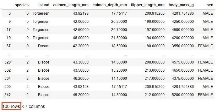
Please note that there are now only 100 samples left after this operation. Here you need to define the factor that is multiplied by the standard deviation. Usually, a value between 2 and 4 is used for this.
Finally, a method of detecting outliers can be used to use percentiles. A certain percentage of values can be assumed from the top or bottom as outliers. Similarly, the value of the percentile used as the boundary of the outlier depends on the distribution of the data. This is the operation that can be performed on the PalmerPenguins dataset:
upper_lim = data['culmen_length_mm'].quantile(.95)
lower_lim = data['culmen_length_mm'].quantile(.05)

no_outliers = data[(data['culmen_length_mm']< upper_lim)&(data['culmen_length_mm']> lower_lim)]
no_outliers
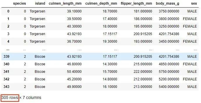
After completing this operation, there are 305 samples in the data set. When using this method, you need to be very careful because it reduces the size of the data set and is highly dependent on the data distribution.
4. Split box
Binning is a simple technique that can group different values into bins. For example, when you want to classify numerical features that look like this:
- 0- 10 -low
- 10- 50 -in
- 50- 100 -high
In this case, replace digital features with categorical features.
However, the classification value can also be classified. For example, you can classify countries/regions by continent:
- Serbia-Europe
- Germany-Europe
- Japan-Asia
- China-Asia
- United States-North America
- Canada-North America
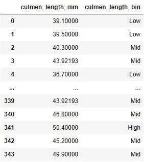
The problem with binning is that it can reduce performance, but it can prevent overfitting and improve the robustness of the machine learning model. This is what it looks like in the code:
bin_data = data[['culmen_length_mm']]
bin_data['culmen_length_bin']= pd.cut(data['culmen_length_mm'], bins=[0,40,50,100], \
          labels=["Low","Mid","High"])
bin_data
5. Zoom
In previous articles, there are often opportunities to understand how scaling can help machine learning models make better predictions. The reason for scaling is simple. If the features are not in the same range, the machine learning algorithm will process them differently. In short, if we have a feature with a value range of 0-10 and another feature with a value range of 0-100, the machine learning algorithm may infer that the second feature is more than the first feature Important because it has a higher value. We already know that this is not always the case. On the other hand, it is unrealistic to expect real data to be in the same range. This is why we use scale to put numerical features in the same range. This standardized data is a common requirement of many machine learning algorithms. Some of them even require that the functions look like standard normally distributed data. We can scale and normalize data in many ways, but before studying them, let’s take a look at a feature of the PalmerPenguins data set "body_mass_g".
scaled_data = data[['body_mass_g']]print('Mean:', scaled_data['body_mass_g'].mean())print('Standard Deviation:', scaled_data['body_mass_g'].std())
-
Mean: 4199.791570763644*
-
Standard Deviation: 799.9508688401579*
In addition, please pay attention to the distribution of this feature:
First, explore scaling techniques that preserve the distribution.
5.1 Standard zoom
This type of scaling removes the mean and scaling data as unit variance. It is defined by the following formula:
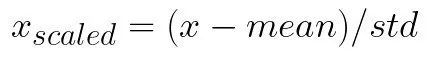
The average is the average of the training samples, and std is the standard deviation of the training samples. The best way to understand it is to observe it in practice. For this, use the SciKit Learn and StandardScaler classes:
standard_scaler =StandardScaler()
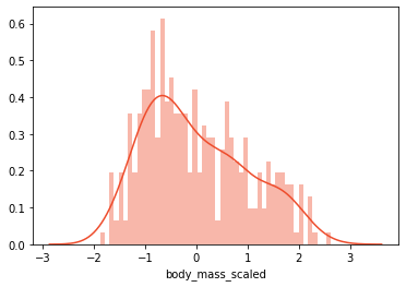
scaled_data['body_mass_scaled']= standard_scaler.fit_transform(scaled_data[['body_mass_g']])print('Mean:', scaled_data['body_mass_scaled'].mean())print('Standard Deviation:', scaled_data['body_mass_scaled'].std())
-
Mean: -1.6313481178165566e-16*
-
Standard Deviation: 1.0014609211587777*
You can see that the original data distribution is retained. However, the data is now between -3 and 3.
5.2 Min-Max zoom ratio (normalized)
The most popular scaling technique is normalization (also called min-max normalization and min-max scaling). It will scale all data in the range of 0 to 1. This technique is defined by the following formula:
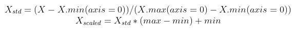
If you use MinMaxScaler in the SciKit learning library:
minmax_scaler =MinMaxScaler()
scaled_data['body_mass_min_max_scaled']= minmax_scaler.fit_transform(scaled_data[['body_mass_g']])print('Mean:', scaled_data['body_mass_min_max_scaled'].mean())print('Standard Deviation:', scaled_data['body_mass_min_max_scaled'].std())
-
Mean: 0.4166087696565679*
-
Standard Deviation: 0.2222085746778217*

The allocation is reserved, but the data is now in the range of 0 to 1.
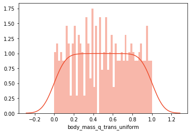
5.3 Quantile conversion
As mentioned, sometimes machine learning algorithms require the data distribution to be uniform or normal. You can use the QuantileTransformer class in SciKit Learn to achieve this. First, this is what it looks like when the data is transformed into a uniform distribution:
qtrans =QuantileTransformer()
scaled_data['body_mass_q_trans_uniform']= qtrans.fit_transform(scaled_data[['body_mass_g']])print('Mean:', scaled_data['body_mass_q_trans_uniform'].mean())print('Standard Deviation:', scaled_data['body_mass_q_trans_uniform'].std())
-
Mean: 0.5002855778903038*
-
Standard Deviation: 0.2899458384920982*
This is the code to put the data in a normal distribution:
qtrans =QuantileTransformer(output_distribution='normal', random_state=0)
scaled_data['body_mass_q_trans_normal']= qtrans.fit_transform(scaled_data[['body_mass_g']])print('Mean:', scaled_data['body_mass_q_trans_normal'].mean())print('Standard Deviation:', scaled_data['body_mass_q_trans_normal'].std())
-
Mean: 0.0011584329410665568*
-
Standard Deviation: 1.0603614567765762*
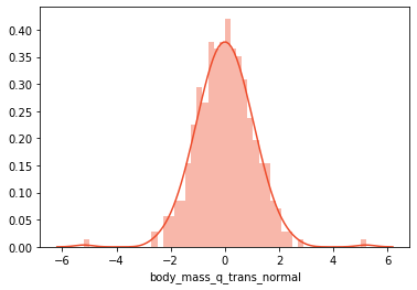
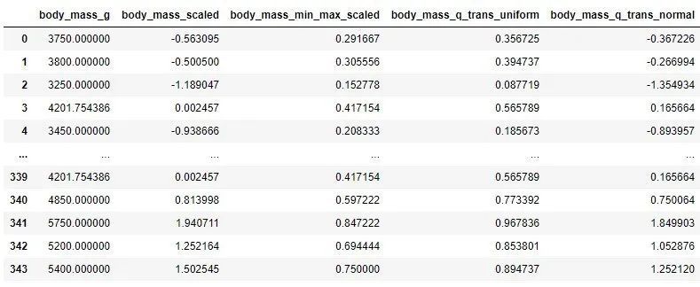
Essentially, the output_distribution parameter is used in the constructor to define the distribution type. Finally, you can observe the zoom values of all features, and have different zoom types:
6. Log conversion
Logarithmic transformation is one of the most popular mathematical transformations of data. Essentially, just apply the log function to the current value. It is important to note that the data must be positive, so if you need to scale or normalize the data in advance. This shift brings many benefits. One of them is that the distribution of data has become more normal. In turn, this helps deal with skewed data and reduces the impact of outliers. This is what it looks like in the code:
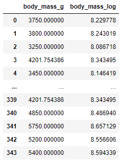
log_data = data[['body_mass_g']]
log_data['body_mass_log']=(data['body_mass_g']+1).transform(np.log)
log_data
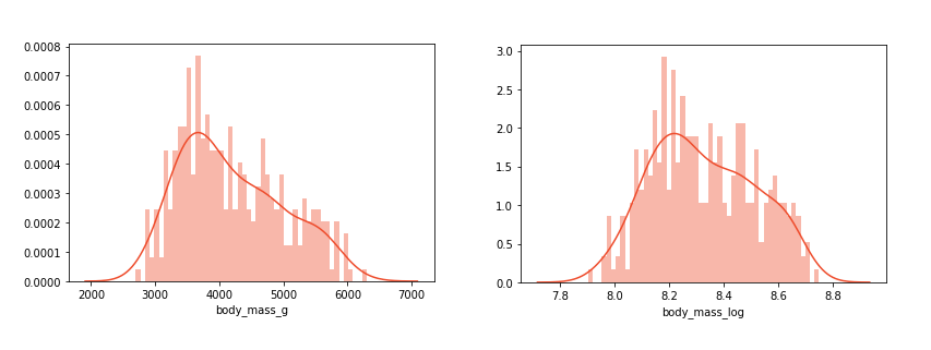
If you check the distribution of the non-transformed data and the transformed data, you can see that the transformed data is closer to the normal distribution:
7. Function selection
The data set from the client is usually very large. Can have hundreds or even thousands of functions. Especially if certain techniques are executed from above. A large number of features can lead to overfitting. In addition, in general, optimizing hyperparameters and training algorithms will take longer. This is why the most relevant features should be selected from the beginning.

Regarding feature selection, there are several techniques, but in this tutorial, only the simplest (and most commonly used) one-univariate feature selection is introduced. The method is based on univariate statistical testing. It uses statistical tests (such as χ2) to calculate how dependent the output features are on each feature in the data set. In this example, SelectKBest is used, which has multiple options when using statistical tests (but the default value is χ2, which is used in this example). This can be done:
feature_sel_data = data.drop(['species'], axis=1)

feature_sel_data["island"]= feature_sel_data["island"].cat.codes
feature_sel_data["sex"]= feature_sel_data["sex"].cat.codes

# Use 3 features
selector =SelectKBest(f_classif, k=3)

selected_data = selector.fit_transform(feature_sel_data, data['species'])
selected_data
array([[39.1,18.7,181.],[39.5,17.4,186.],[40.3,18.,195.],...,[50.4,15.7,222.],[45.2,14.8,212.],[49.9,16.1,213.]])
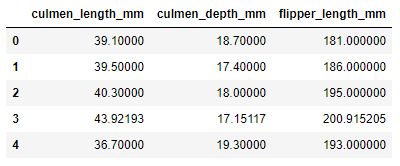
Using the hyperparameter k, the three most influential features in the data set are defined. The output of this operation is a NumPy array containing the selected elements. To put it in a pandas Dataframe, you need to do the following:
selected_features = pd.DataFrame(selector.inverse_transform(selected_data),
         index=data.index,
         columns=feature_sel_data.columns)

selected_columns = selected_features.columns[selected_features.var()!=0]
selected_features[selected_columns].head()
8. Function grouping
So far, in terms of so-called "cleanliness", the observed data set is almost perfect. This means that each element has its own column, each observation is a row, and each type of observation unit is a table. However, sometimes the observations are distributed in several rows. The goal of functional grouping is to concatenate these rows into one row and then use these summarized rows. The main question in doing this is which aggregate function will be applied to the features. This is especially complicated for classification features.
As mentioned, the PalmerPenguins dataset is very typical, so the following example is only used to illustrate the code that can be used for this operation:
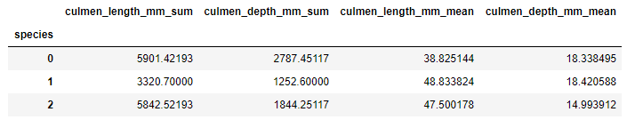
grouped_data = data.groupby('species')

sums_data = grouped_data['culmen_length_mm','culmen_depth_mm'].sum().add_suffix('_sum')
avgs_data = grouped_data['culmen_length_mm','culmen_depth_mm'].mean().add_suffix('_mean')

sumed_averaged = pd.concat([sums_data, avgs_data], axis=1)
sumed_averaged
Here, the data is grouped by spices value, and two new features with sum and average value are created for each value.
9. Function split
Sometimes data is not connected across rows, but across columns. For example, suppose there is a list of names in one of the functions:
data.names
0 Andjela Zivkovic
1 Vanja Zivkovic
2 Petar Zivkovic
3 Veljko Zivkovic
4 Nikola Zivkovic
Therefore, if you only want to extract the name from this function, you can do the following:
data.names
0 Andjela
1 Vanja
2 Petar
3 Veljko
4 Nikola
This technique is called feature segmentation and is usually used for string data.
in conclusion
In this article, I have the opportunity to explore the 9 most commonly used feature engineering techniques.
Recommended Posts