matplotlib of python drawing module

Last week, fio hard disk performance tests were conducted on certain online disks. After the test is completed, the results need to be drawn into images for display. I looked up the usage of fio's own commands fio_generate_plot and fio2gnuplot tools on the official website, and found out how to draw images. In a single scene, you can indeed use these two tools to draw hard disk performance images, but there is a problem Yes, if you want to compare the differences of the images drawn in multiple scenes, the drawing tools that come with fio are somewhat difficult to implement, but they can be implemented. For example:

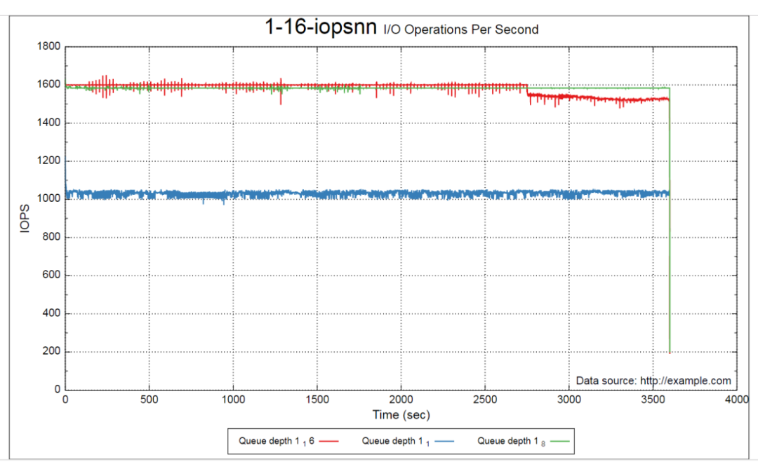
As shown in the figure, the disk iodepth is unchanged, and numjobs is drawn in three different scenarios (1, 8, 16). How to draw it, forgive me for not finding a way for the time being. This is an image drawn by predecessors.

So in order to solve this problem in a different way of thinking, I searched for python drawing methods and found a way to draw multiple graphs using the python matplotlib module. If your computer does not have this module, please use:

pip install matplotlib command to install.

Take a look at the way matplotlib draws curves:

# /usr/bin/env python
# - *- coding=utf-8-*-import matplotlib.pyplot as plt

def PlotDemo1():
 fig = plt.figure()  #The figure object can be seen as the entire chart. Add multiple subgraphs on top of the figure chart, and then draw points and lines on the subgraphs
 # By add_Subplot adds subplots (returns an axes axis), this method requires three parameters, namely: numrows, numcols,fignum. Among them, there are a total of numrows*numcols subgraphs,
 # Divide the chart into N rows*M column, fignum identifies the order of the subgraph, and its range is from 1 to numrows*numcols. In the above example 1,1,1 means that the drawing object has only 1 subgraph, which is 1*1 type
 ax = fig.add_subplot(1,1,1)
 ax.plot([1,2,3,4])   #Specify the ordinate, the number of abscissas will be automatically set equal to the number of ordinates, starting from 0, that is, the abscissa will become[0,1,2,3]
 ax.plot([1,2,3,4],[2,3,4,5])  #Specify the abscissa and ordinate to draw another curve
 plt.show()PlotDemo1()

Here I have drawn the simplest two curves. The ax variable can continue to add the x array and y array that need to be plotted, so that several lines can be drawn in one graph. Look at the result graph drawn by the above code:

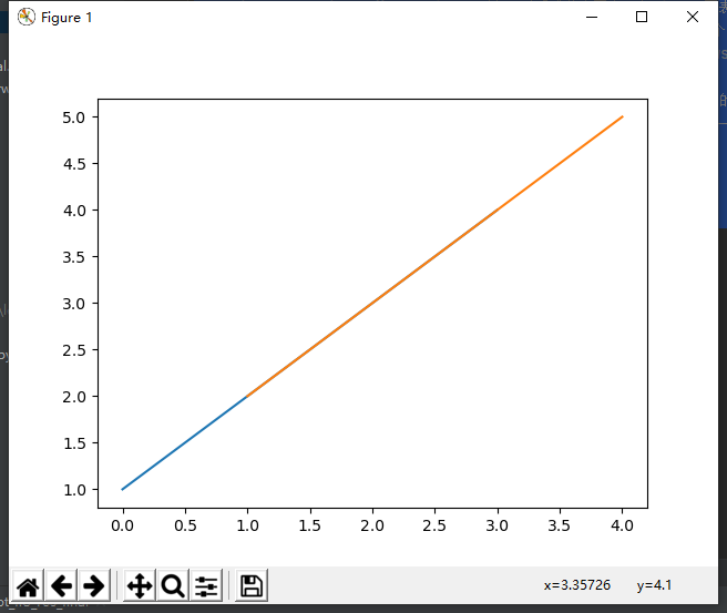
You can see that there are two lines:

The first is the blue line, which is:

ax.plot([1,2,3,4])

The parameter passed in this command represents the value of the ordinate. Because the abscissa is not passed, the abscissa starts from 0 by default and increases in 1-bit units.

The second is the orange line:

ax.plot([1,2,3,4],[2,3,4,5])

The first array of this command is the x-axis array, and the second array is the Y-axis array

The two lines partially overlap, so they look like a straight line.

With this drawing idea, we can put the points we need to draw in two lists, one as the abscissa and the other as the ordinate, so that we can draw the image we want, about the image The title, description of the horizontal and vertical coordinates, icons, etc., can all be enriched with the corresponding function. For specific drawing methods, please refer to the more detailed module descriptions on the Internet. Here I will provide an idea, I hope it will be helpful to everyone.

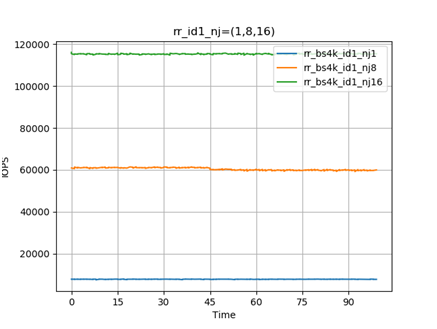
Finally, the above graphs of disk performance drawn with python can be compared with the above graphs: